JPL: Slowdown of North Atlantic sub-polar gyre found by Jason-1; sea level changes 1993-2008

PIA11002: Portrait of a Warming Ocean and Rising Sea Levels:
Trend of Sea Level Change 1993-2008
Target Name: Earth
Is a satellite of: Sol (our sun)
Mission: Jason-1 (TOPEX/Poseidon)
Spacecraft: Jason-1 (TOPEX/Poseidon)
Instrument: Altimeter
Product Size: 919 samples x 699 lines
Produced By: JPL
Full-Res TIFF: PIA11002.tif (644.9 kB)
Full-Res JPEG: PIA11002.jpg (104.2 kB)

Click on the image to download a moderately sized image in JPEG format (possibly reduced in size from original).
Original Caption Released with Image:

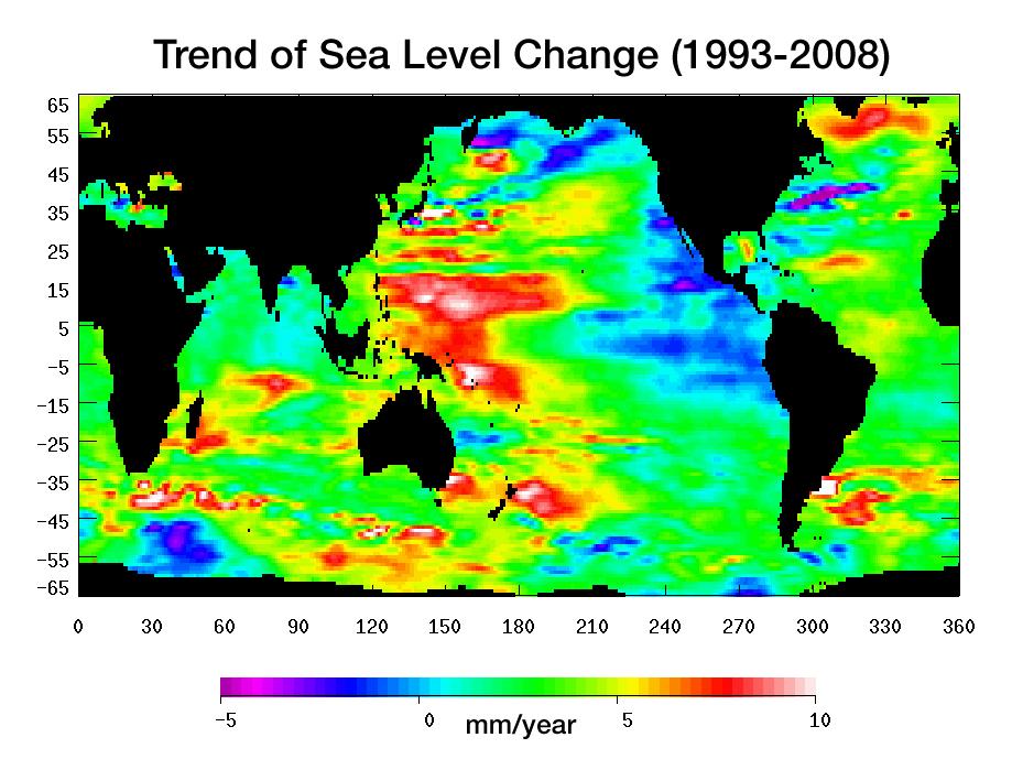
Warming water and melting land ice have raised global mean sea level 4.5 centimeters (1.7 inches) from 1993 to 2008. But the rise is by no means uniform. This image, created with sea surface height data from the Topex/Poseidon and Jason-1 satellites, shows exactly where sea level has changed during this time and how quickly these changes have occurred.

It’s also a road map showing where the ocean currently stores the growing amount of heat it is absorbing from Earth’s atmosphere and the heat it receives directly from the Sun. The warmer the water, the higher the sea surface rises. The location of heat in the ocean and its movement around the globe play a pivotal role in Earth’s climate.

Light blue indicates areas in which sea level has remained relatively constant since 1993. White, red, and yellow are regions where sea levels have risen the most rapidly—up to 10 millimeters per year—and which contain the most heat. Green areas have also risen, but more moderately. Purple and dark blue show where sea levels have dropped, due to cooler water.

The dramatic variation in sea surface heights and heat content across the ocean are due to winds, currents and long-term changes in patterns of circulation. From 1993 to 2008, the largest area of rapidly rising sea levels and the greatest concentration of heat has been in the Pacific, which now shows the characteristics of the Pacific Decadal Oscillation (PDO), a feature that can last 10 to 20 years or even longer.

In this “cool” phase, the PDO appears as a horseshoe-shaped pattern of warm water in the Western Pacific reaching from the far north to the Southern Ocean enclosing a large wedge of cool water with low sea surface heights in the eastern Pacific. This ocean/climate phenomenon may be caused by wind-driven Rossby waves. Thousands of kilometers long, these waves move from east to west on either side of the equator changing the distribution of water mass and heat.

This image of sea level trend also reveals a significant area of rising sea levels in the North Atlantic where sea levels are usually low. This large pool of rapidly rising warm water is evidence of a major change in ocean circulation. It signals a slow down in the sub-polar gyre, a counter-clockwise system of currents that loop between Ireland, Greenland and Newfoundland.

Such a change could have an impact on climate since the sub-polar gyre may be connected in some way to the nearby global thermohaline circulation, commonly known as the global conveyor belt. This is the slow-moving circulation in which water sinks in the North Atlantic at different locations around the sub-polar gyre, spreads south, travels around the globe, and slowly up-wells to the surface before returning around the southern tip of Africa. Then it winds its way through the surface currents in the Atlantic and eventually comes back to the North Atlantic.

It is unclear if the weakening of the North Atlantic sub-polar gyre is part of a natural cycle or related to global warming.

This image was made possible by the detailed record of sea surface height measurements begun by Topex/Poseidon and continued by Jason-1. The recently launched Ocean Surface Topography Mission on the Jason-2 satellite (OSTM/Jason-2) will soon take over this responsibility from Jason-1. The older satellite will move alongside OSTM/Jason-2 and continue to measure sea surface height on an adjacent ground track for as long as it is in good health.

Topex/Poseidon and Jason-1 are joint missions of NASA and the French space agency, CNES. OSTM/Jason-2 is collaboration between NASA; the National Oceanic and Atmospheric Administration; CNES; and the European Organisation for the Exploitation of Meteorological Satellites. JPL manages the U.S. portion of the missions for NASA's Science Mission Directorate, Washington, D.C.

Image Credit:
NASA/JPL
Link to article: http://photojournal.jpl.nasa.gov/catalog/PIA11002

WAIS: Short-Term Spikes, Long-Term Warming Linked to Tropical Pacific

Antarctic Climate: Short-Term Spikes, Long-Term Warming Linked to Tropical Pacific

August 12, 2008

BOULDER—Dramatic year-to-year temperature swings and a century-long warming trend across West Antarctica are linked to conditions in the tropical Pacific Ocean, according to a new analysis of ice cores conducted by scientists at the National Center for Atmospheric Research (NCAR) and the University of Washington (UW). The findings show the connection of the world's coldest continent to global warming, as well as to periodic events such as El Niño.

El Niño develops across the tropical Pacific

When a strong El Niño develops across the tropical Pacific, it can influence weather and climate as far away as the southern polar region. This occurs via a "wave train" of areas with unusually high or low pressure in the upper atmosphere (Hs and Ls) that leads to warmer-than-normal temperatures in West Antarctica. Bright reds near the equator show the unusually warm sea-surface temperatures (SSTs) associated with an El Niño during 1940-41. There are no SST data for that period for the portions of the Southern Ocean shown here. Analysis of ice cores drilled in West Antarctica (red dots) reveals that air temperatures there warmed by as much as 10°F as this 3-year-long El Niño unfolded, then dropped by as much as 13°F afterward. [ENLARGE] (image by Steve Deyo, ©UCAR)

"As the tropics warm, so too will West Antarctica," says NCAR's David Schneider, who conducted the research with UW's Eric Steig. "These ice cores reveal that West Antarctica's climate is influenced by atmospheric and oceanic changes thousands of miles to the north."

The research appears this week in the online Early Edition of Proceedings of the National Academy of Sciences. The work was supported by the National Science Foundation, NCAR's sponsor.

Scientists are keenly interested in whether warming will destabilize the West Antarctic ice sheet over a period of decades or centuries. The ice sheet covers an area the size of Mexico, averages about 6,500 feet deep, and, if melted, would raise global sea levels by about 8 to 16 feet (2.5-5 meters).

Antarctica's climate is difficult to study, partly because there are few observations of this vast and remote region and partly because the cold, dry atmosphere is unlike that of the other six continents. Scientists previously determined that Antarctica overall probably warmed by about 0.4 degrees Fahrenheit (0.2 degrees Celsius) in the last century. But it has not been apparent until now that low-lying West Antarctica is more responsive to global warming trends than East Antarctica, where wind patterns have largely kept out comparatively warm air.

Schneider and Steig estimate that West Antarctica warmed about 1.6 degrees F (0.9 degrees C) over the 20th century. That is slightly more than the global average of about 1.3 degrees F (0.7 degrees C). Because of the large swings in annual temperature during the 1930s and 1940s, there is a considerable margin of uncertainty in the century-long estimate, says Schneider. He notes that there is increased confidence that warming has occurred since 1950, averaging about 0.8 degree F (0.4 degrees C) per decade.

David Schneider

David Schneider (photo by David Hosansky, ©UCAR)

The new set of cores analyzed by Schneider and Steig comes from a relatively snowy part of the continent. This provides enough detail for scientists to infer year-to-year temperature changes. The data show that the Antarctic climate is highly responsive to changes in the Pacific. For example, during a major El Niño event from 1939 to 1942, temperatures in West Antarctica rose by about 6 to 10 degrees F (3-6 degrees C), and then dropped by an estimated 9 to 13 degrees F (5-7 degrees C) over the next two years. El Niño is a periodic shift in air pressure accompanied by oceanic warming in the tropical Pacific.

Although the heart of El Niño's oceanic warming is in the tropical Pacific, it often fosters a circulation pattern that pushes relatively mild, moist air toward West Antarctica, where it can temporarily displace much colder air. As a result, West Antarctica has one of the world's most variable climates.

"These results help put Antarctica's recent climate trends into a global context," says Schneider.

Steig adds that while the influence of tropical climate on West Antarctica climate was not unknown, "these results are the first to demonstrate that we can unambiguously detect that influence in ice core records."

Decoding the climate record

Ice-core analysis is critical for understanding the climate of West Antarctica. Few weather stations existed before the 1950s, and even satellite readings can be unreliable because of the difficulty in distinguishing clouds from snow cover.

To reconstruct climate trends over the last century, Schneider and Steig analyzed ice cores collected from eight locations across West Antarctica. They measured heavy and light stable isotopes of oxygen and hydrogen, the elements that make up the ice itself. During warm episodes, the heavy isotopes are more common because of a number of processes, such as a reduction in condensation that would otherwise remove them.

The ice cores for the study were collected from 2000 to 2002 during the U.S. International Trans-Antarctic Scientific Expedition, which Schneider and Steig participated in.

Link to article at NCAR: http://www.ucar.edu/news/releases/2008/antarcticwarming.jsp

NSIDC: Arctic Sea ice decline accelerates, Amundsen's Northwest Passage opens

Arctic sea ice reflects sunlight, keeping the polar regions cool and moderating global climate. According to scientific measurements, Arctic sea ice has declined dramatically over at least the past thirty years, with the most extreme decline seen in the summer melt season.

Read timely scientific analysis year-round below. We provide an update during the first week of each month, or more frequently as conditions warrant.

Please credit the National Snow and Ice Data Center for image or content use unless otherwise noted beneath each image.

August 11, 2008

Sea ice decline accelerates, Amundsen's Northwest Passage opens

Sign up for the Arctic Sea Ice News RSS feed for automatic notification of analysis updates.

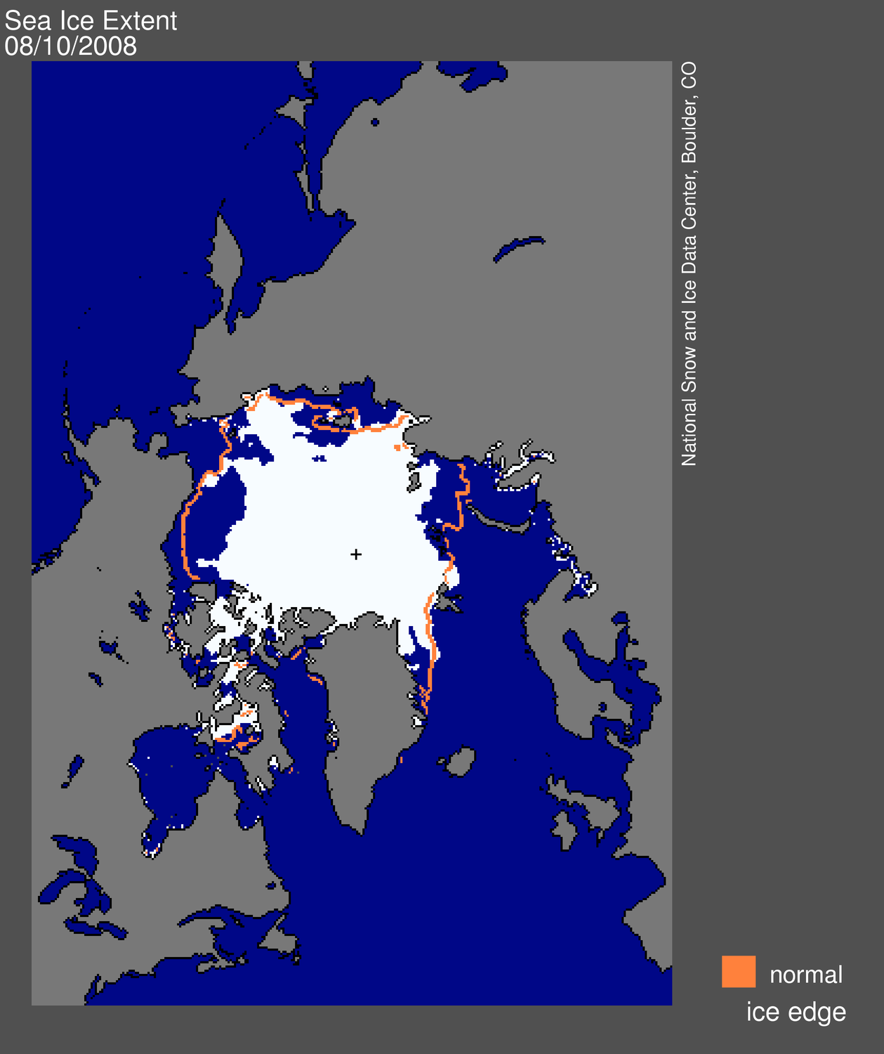
The pace of sea ice loss sharply quickened in the past ten days, triggered by a series of strong storms that broke up thin ice in the Beaufort and Chukchi Seas. Amundsen's historic Northwest Passage is opening up; the wider and deeper route through Parry Channel is currently still clogged with ice.

Note: Analysis updates, unless otherwise noted, now show a single-day extent value for Figure 1, as opposed to the standard monthly average. While monthly average extent images are more accurate in understanding long-term changes, the daily images are helpful in monitoring sea ice conditions in near-real time.

Map of sea ice from space, showing sea ice, continents, ocean
Figure 1. Daily Arctic sea ice extent for August 10, 2008, was 6.54 million square kilometers (2.52 million square miles). The orange line shows the 1979 to 2000 average extent for that day. The black cross indicates the geographic North Pole. Sea Ice Index data. About the data.
—Credit: National Snow and Ice Data Center

High-resolution image

Overview of conditions

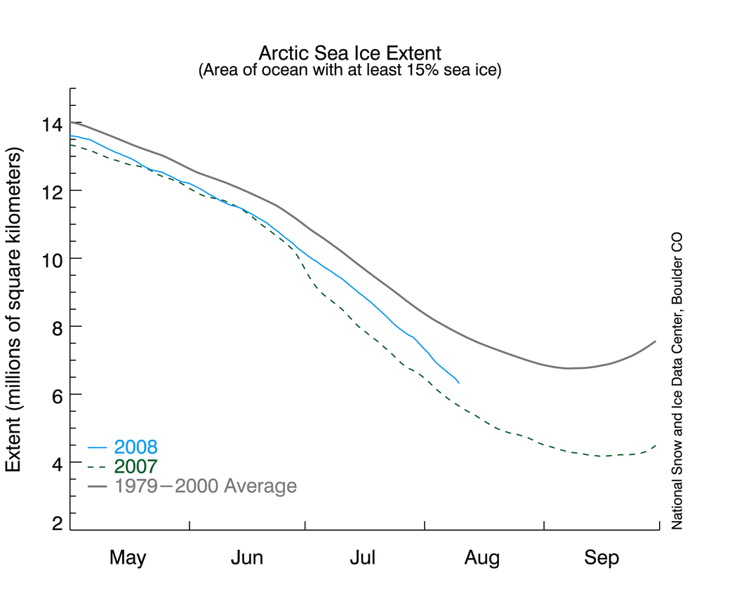
Arctic sea ice extent on August 10 was 6.54 million square kilometers (2.52 million square miles), a decline of 1 million square kilometers (390,000 square miles) since the beginning of the month. Extent is now within 780,000 square kilometers (300,000 square miles) of last year's value on the same date and is 1.50 million square kilometers (580,000 square miles) below the 1979 to 2000 average.

Graph with months on x axis and extent on y axis
Figure 2. Daily sea ice extent; the blue line indicates 2008; the gray line indicates extent from 1979 to 2000; the dotted green line shows extent for 2007. Sea Ice Index data.
—Credit: National Snow and Ice Data Center

High-resolution Image

Conditions in context

Ice extent has begun to decline sharply. The decline rate surged to -113,000 square kilometers per day on August 7 and as of August 10 was -103,000 square kilometers per day. This compares to the long-term average decline of -76,000 square kilometers per day for this time of year. Normally, the peak decline rate is in early July.

Many of the areas now seeing a rapid retreat saw an early melt onset (see July 2, 2008); this helped set the stage for rapid retreat (July 17 and April 7). However, the more fundamental issue is that these regions started the melt season covered with thin first-year ice, which is especially vulnerable to melting out completely. Thin ice is also vulnerable to breakup by winds; the last ten days have seen a windy, stormy pattern that has accelerated the ice loss.

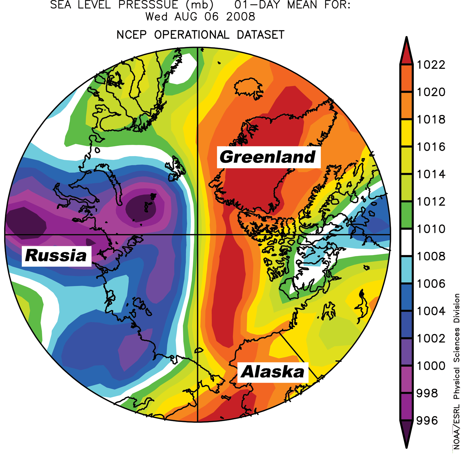
Satellite view of Arctic shwoing color bandsFigure 3. Sea-level pressure for August 8, 2008, shows a weather pattern favoring ice melt. Areas of high pressure are shown in yellow and red; areas of low pressure are shown in blue and purple.
—Credit: From National Snow and Ice Data Center courtesy Climate Diagnostic Center

High-resolution image

Storms trigger increased melt

A series of storms north of Alaska and Siberia in late July and early August have helped break up the thin ice and have brought warm southerly winds into the region.

Subsequently, a pattern has developed with high pressure over the Beaufort Sea and low pressure over the Laptev and East Siberian Seas (Figure 3). In accord with Buys Ballot's Law, this pattern has brought southerly winds to the region, enhancing melt, breaking up ice, and pushing the ice edge northward.

view of North Passage area from space
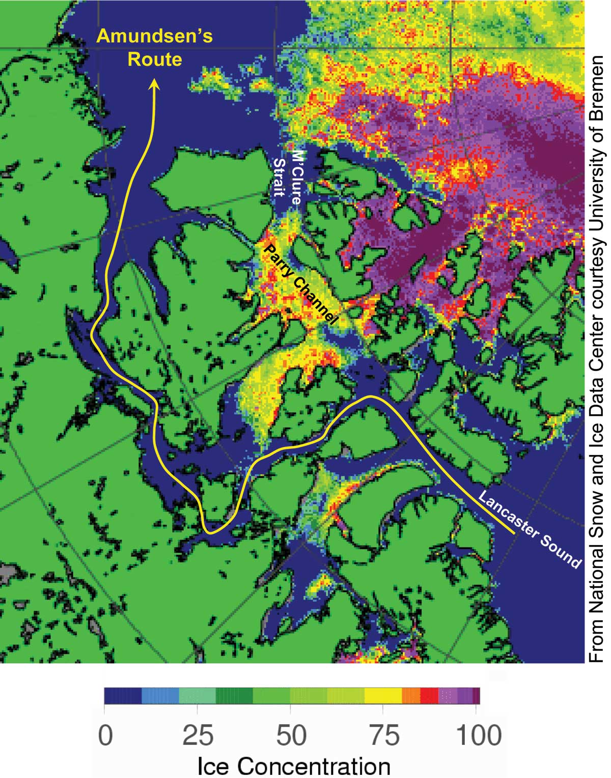
Figure 4. Passive-microwave satellite data shows ice concentration on August 10, 2008, over the Northwest Passage region. The yellow line indicates Amundsen's historic route through the passage. NASA AMSR-E data.
—Credit: From National Snow and Ice Data Center courtesy University of Bremen

High-resolution image

Opening of Amundsen's Northwest Passage

The Northwest Passage that Roald Amundsen navigated with great difficulty starting in 1903 is opening for the second year in a row, as shown in the AMSR-E sea ice product from the University of Bremen (Figure 4).

The most recent operational analysis from the Canadian Ice Service and the U.S. National Ice Center on August 8 showed a small section of Amundsen’s historic path still blocked by a 50-kilometer (31-mile) stretch of sea ice, although that should melt within the next few days.

Amundsen’s route requires sailing through treacherous narrow and shallow channels, making it impractical for deep-draft commercial ships. The more important northern route, through the wide and deep Parry Channel, is still ice-clogged. The northern route opened in mid-August last year; it may still open up before the end of this year's melt season.

For previous analysis, please see the drop-down menu under Archives in the right navigation at the top of this page.

NASA logoNSIDC scientists provide Arctic Sea Ice News & Analysis, with partial support from NASA.

Thomas L. Friedman: Flush with Energy

Flush With Energy

by THOMAS L. FRIEDMAN, August 9, 2008, Copenhagen
Thomas L. Friedman (credit Fred R. Conrad/The New York Times).

The Arctic Hotel in Ilulissat, Greenland, is a charming little place on the West Coast, but no one would ever confuse it for a Four Seasons — maybe a One Seasons. But when my wife and I walked back to our room after dinner the other night and turned down our dim hallway, the hall light went on. It was triggered by an energy-saving motion detector. Our toilet even had two different flushing powers depending on — how do I say this delicately — what exactly you’re flushing. A two-gear toilet! I’ve never found any of this at an American hotel. Oh, if only we could be as energy efficient as Greenland!

A day later, I flew back to Denmark. After appointments here in Copenhagen, I was riding in a car back to my hotel at the 6 p.m. rush hour. And boy, you knew it was rush hour because 50 percent of the traffic in every intersection was bicycles. That is roughly the percentage of Danes who use two-wheelers to go to and from work or school every day here. If I lived in a city that had dedicated bike lanes everywhere, including one to the airport, I’d go to work that way, too. It means less traffic, less pollution and less obesity.

What was most impressive about this day, though, was that it was raining. No matter. The Danes simply donned rain jackets and pants for biking. If only we could be as energy smart as Denmark!

Unlike America, Denmark, which was so badly hammered by the 1973 Arab oil embargo that it banned all Sunday driving for a while, responded to that crisis in such a sustained, focused and systematic way that today it is energy independent. (And it didn’t happen by Danish politicians making their people stupid by telling them the solution was simply more offshore drilling.)

What was the trick? To be sure, Denmark is much smaller than us and was lucky to discover some oil in the North Sea. But despite that, Danes imposed on themselves a set of gasoline taxes, CO2 taxes and building-and-appliance efficiency standards that allowed them to grow their economy — while barely growing their energy consumption — and gave birth to a Danish clean-power industry that is one of the most competitive in the world today. Denmark today gets nearly 20 percent of its electricity from wind. America? About 1 percent.

And did Danes suffer from their government shaping the market with energy taxes to stimulate innovations in clean power? In one word, said Connie Hedegaard, Denmark’s minister of climate and energy: “No.” It just forced them to innovate more — like the way Danes recycle waste heat from their coal-fired power plants and use it for home heating and hot water, or the way they incinerate their trash in central stations to provide home heating. (There are virtually no landfills here.)

There is little whining here about Denmark having $10-a-gallon gasoline because of high energy taxes. The shaping of the market with high energy standards and taxes on fossil fuels by the Danish government has actually had “a positive impact on job creation,” added Hedegaard. “For example, the wind industry — it was nothing in the 1970s. Today, one-third of all terrestrial wind turbines in the world come from Denmark.” In the last 10 years, Denmark’s exports of energy efficiency products have tripled. Energy technology exports rose 8 percent in 2007 to more than $10.5 billion in 2006, compared with a 2 percent rise in 2007 for Danish exports as a whole.

“It is one of our fastest-growing export areas,” said Hedegaard. It is one reason that unemployment in Denmark today is 1.6 percent. In 1973, said Hedegaard, “we got 99 percent of our energy from the Middle East. Today it is zero.”

Frankly, when you compare how America has responded to the 1973 oil shock and how Denmark has responded, we look pathetic.

“I have observed that in all other countries, including in America, people are complaining about how prices of [gasoline] are going up,” Denmark’s prime minister, Anders Fogh Rasmussen, told me. “The cure is not to reduce the price, but, on the contrary, to raise it even higher to break our addiction to oil. We are going to introduce a new tax reform in the direction of even higher taxation on energy and the revenue generated on that will be used to cut taxes on personal income — so we will improve incentives to work and improve incentives to save energy and develop renewable energy.”

Because it was smart taxes and incentives that spurred Danish energy companies to innovate, Ditlev Engel, the president of Vestas — Denmark’s and the world’s biggest wind turbine company — told me that he simply can’t understand how the U.S. Congress could have just failed to extend the production tax credits for wind development in America.

Why should you care?

“We’ve had 35 new competitors coming out of China in the last 18 months,” said Engel, “and not one out of the U.S.”

[A version of this article appeared in print on August 10, 2008, on page WK11 of the New York edition.]

Link to article: http://www.nytimes.com/2008/08/10/opinion/10friedman1.html

UPDATE: Arctic Sea ice well on its way to disappearing this summer -- Part IV

BLOGGER'S NOTE, August 11: vast stretches of the Arctic Sea ice are quite thin -- in the range of 10-20 cm only -- and if you look down at the bottom of this post, you will see a graphic of the 2-m temperatures in the Northern Hemisphere that shows that temperatures are very high in northwestern Canada and Siberia near the Arctic Sea; thus, it seems that we can expect much of the very thin ice to melt in the next few days, unless colder air moves in.

BLOGGER'S NOTE, August 10: for a new set of graphics that give much more detailed information, go to the bottom of this particular post.

BE SURE TO CLICK ON THE IMAGES TO ENLARGE THE DETAIL.


From Polar View at the Technical University of Denmark (http://www.seaice.dk/):
BELOW: Graphic from August 10, 2008:


From the Cryosphere Today site (run by the Universities of Illinois and Colorado), a comparison of the Arctic on August 9 and July 22, 2007 and 2008:


Go to this link and put in dates for comparison -- the most recent day is usually available before the evening: http://igloo.atmos.uiuc.edu/cgi-bin/test/print.sh


The graphics below are from NOAA of global sea surface temperature anomalies on August 7 and July 24, 2008.


Link to updated graphics: http://www.osdpd.noaa.gov/PSB/EPS/SST/climo.html


The image below is a NOAA graphic of the 500-hPa height anomalies in the Northern Hemisphere on June 9, 2008. Click on the link below the graphic to see the most recent 30-day animation.


Link to past 30-days' animation: http://www.cpc.noaa.gov/products/intraseasonal/z500_nh_anim.shtml


BELOW
: from Bremen University, a graphic of the Arctic Sea Ice extent, on August 10, 2008 (be sure to click on it in order to see the detail):

Link to the graphics above (occasionally data are missing and are represented by grey areas -- normally, these areas will be filled in by the morning of the following day): http://www.iup.uni-bremen.de:8084/amsr/amsre.html


ABOVE: visual ice cover, August 10, 2008.
BELOW: July 24, 2008 (from Bremen University).


Link to updated images: http://www.iup.uni-bremen.de:8084/amsr/arctic_AMSRE_visual.png


Link to photos (NOTE: to see photos from other days from 2008, change the 222 to the number of the day that you want, e.g., 222 is August 9th, and 208 is July 26th, and so forth):
http://manati.orbit.nesdis.noaa.gov/ice_image21/D08222.NHEAVEH.GIF


BELOW
: from the Japanese Aerospace Exploration Agency, a graphic of Arctic Sea ice extent for the current and past years, August 9, 2008.
The latest value : 6,417,656 km2:

Link to graphic: http://www.ijis.iarc.uaf.edu/en/home/seaice_extent.htm


BELOW: National Snow and Ice Data Center graph of Arctic Sea ice extent, August 10, 2008:


Link to graph: http://nsidc.org/data/seaice_index/images/daily_images/N_timeseries.png


I find the image below fascinating (and it is the scariest of all):


Link to updated TLT channel temperature anomalies graph (NOTE: often due to volume of traffic it is not possible to access the link -- try again later):
http://www.remss.com/msu/msu_data_description.html#figures


And, below, find an animation of global surface temperature anomalies for the past 30 days -- most disturbing are the anomalies occurring at Antarctica many of which are much higher than 20 C.


Link to animation above: http://www.cdc.noaa.gov/map/images/fnl/sfctmpmer_01a_30frames.fnl.anim.html
ABOVE: image from August 4th, 2008.

BELOW, temperature map of the Arctic (first click on the link below the picture, then click on the yellow dots to see weather conditions -- some dots are inactive):


Link to map: http://www.athropolis.com/map2.htm


BELOW: graphic of ice thickness (http://seaice.bplaced.net/gfs.html):


BELOW: graphic of 2-meter height temperatures (http://seaice.bplaced.net/gfs.html):

Roger Pielke, Jr.: NCAR's NSF Budget -- The Real Facts

NCAR’s NSF Budget: The Real Facts

August 9th, 2008

Posted by: Roger Pielke, Jr.

On Friday, NCAR put out a press release with the following claims:

The National Center for Atmospheric Research, like many universities and other research institutions in the United States, continues to face extraordinary budget pressures, due to the decreases in real terms in federal funding for science. Over the past five years we have had to lay off over 50 people and have lost another 60 due to attrition, totaling roughly 12% of our NSF-supported staff, because of sub-inflationary National Science Foundation funding.

Several claims in this statement are misleading and even outright wrong.

First, have there been “decreases in real terms in federal funding for science?” No, there have not. The following figure from AAAS (PDF) shows that after adjusting for inflation budgets have been flat for the past several years, but certainly not decreasing. Nondefense science budgets have actually been increasing slightly after inflation.

That federal science budgets were going to plateau (at least) was fairly obvious in 2004. At the time I wrote:

Few seem to be aware that over the past decade S&T has experienced a second golden age, at least as measured by federal funding, which has increased dramatically in recent years at a pace not seen since the 1960s. But this second golden age is now ending and the consequences for science politics and policies are likely to be profound.

Second, NCAR’s press release also asserts that with respect to the NCAR allocation from NSF:

NSF and all of the government agencies that support science have faced similar budgetary stringencies. Over the past five years we have had to make painful cuts in all areas of our scientific and facilities programs—including climate, weather, atmospheric chemistry, solar physics and certain computational and observational facilities and services. . . Unfortunately, this year we are projecting a shortfall of $8 million (about 10%) in our NSF base budget and must plan for a worst-case shortfall next year of roughly $10 million.

Sounds dire, but the actual NSF data tells a very different story. The following shows the NSF allocation to NCAR for 2005-2008 (data from the NSF Budget www site) both in current and constant 2008 dollars (adjusted using the official implicit GDP price deflator).

The data show that in real terms the NCAR 2008 budget is about $0.3 million less than it was in 2005. How this situation translates into a shortfall of some $8 million — implying a need for 2005-2008 growth to be 10% above inflation — is beyond my reckoning. Perhaps NCAR has confused a lack of growth in desired spending with a budget cut, but who knows. Similarly, how a budget that grows almost exactly with inflation results in a loss of 12% of NSF-funded NCAR employees boggles the mind. They are either giving out huge raises or moving their spending away from people to equipment (like to the annual upkeep of an earmarked airplane, but I digress). Who knows what is going on at NCAR, but the spin and misdirection are not good signs.

Link to Dr. Pielke's blog: http://sciencepolicy.colorado.edu/prometheus/date/2008/08/09

Roger Pielke, Jr.'s take on the budget cuts at NCAR

From Roger Pielke, Jr.'s blog concerning the budget cuts at NCAR:

"Tone Deaf Damage Control

August 9th, 2008

Posted by: Roger Pielke, Jr.

I find this hard to believe. As readers of this blog know, earlier this week NCAR administrator Eric Barron made the difficult decision to cut the organization’s Center for Capacity Building, which is focused on helping developing countries adapt to climate. The decision prompted a flurry of compaints and international media coverage.

I was thus surprised to see the email copied below (which was sent to a bunch of people) from Eric and UCAR Vice President Jack Fellows:

From: “Jack Fellows”
Date: August 5, 2008 7:36:07 PM EDT
To: Bierbaum Rosina , peter backlund , Kelly Redmond , kelly redmond , Brad Udall , david yates , Jonathan Overpeck , kathy hibbard , linda mearns , mary hayden , lawrence buja , tom warner , kathleen miller , philip mote , caitlin simpson , Chester J Koblinsky , lisa goddard , Nolan Doesken , Alan Robock , Mark Abbott , “Mark Z. Jacobson” , dan vimont , Anthony Janetos , greg carbone , “Rudnicki Mark” , Keith Talbert Ingram , brian oneill , Paty Romero Lankao , Liz Moyer , david battisti , urc
Cc: eric barron
Subject: 2008 AGU Fall Session on Climate Adaptation

Eric Barron and I are putting together the AGU session described below. If you have put one of these AGU sessions together, you know that I can’t promise you that it will be an oral session or the day/time it will happen, and you are restricted to no more than 3 first author abstracts for the Fall AGU mtg. That said, we’d love to have you participate in this session. Let me know if you are interested by _17 August _so I can meet an 18 Aug AGU deadline. If you can’t participate but know of a great person, please forward this email on to them. Thanks. This is a large email list, so pls just respond to my email address. Jack

Description: PA03: How Can the Science Community Help Local and Regional Decision Makers Who are Exploring or Implementing Adaptation Options to Climate Change? All weather is local! The same will be true regarding adapting to climate change. This session will examine how local universities and decision makers are working together to adapt to anticipated climate change impacts and explore how these independent activities might be networked together into a “national adaptation network or model”. NOTE: we are primarily interested in people who have really interesting policy research or a project that is partnering with local and regional decision makers to deal with climate adaptation, mitigation, or even geoengineering.

Note that the time stamp of the email is after the brouhaha started about the decision to cut CCB. This appears to be an exercise in damage control — “We really care about adaptation, no really, we do. Look we sponsored a session at AGU!” — since neither Barron or Fellows have even done any work in adaptation (and to my knowledge Fellows is an administrator, not at all a researcher).

Let me try my hand at answering the question that they pose:

How Can the Science Community Help Local and Regional Decision Makers Who are Exploring or Implementing Adaptation Options to Climate Change? . . . This session will examine how local universities and decision makers are working together to adapt to anticipated climate change impacts and explore how these independent activities might be networked together into a “national adaptation network or model”.

First thing, don’t cut a program with a 34-year track record of success in doing exactly this. Are these guys serious that they now want to discuss how to recreate the functions of the NCAR CCB at an AGU session? Seriously?

I’d love to give NCAR/UCAR management the benefit of the doubt and believe that they have a rigorous method for setting priorities and making cuts. But not only is this sort of tone deaf damage control/spin insulting to the actual adaptation research community, but a sign that NCAR/UCAR may have a management problem rather than a budget problem.