A quick post for commentary on the new Solomon et al paper in Science Express. We’ll try and get around to discussing this over the weekend, but in the meantime I’ve moved some comments over. There is some commentary on this at DotEarth, and some media reports on the story – some good, some not so good. It seems like a topic that is ripe for confusion, and so here are a few quick clarifications that are worth making. First of all, this is a paper about internal variability of the climate system in the last decade, not on additional factors that drive climate. Second, this is a discussion about stratospheric water vapour (10–15 km above the surface), not water vapour in general. Stratospheric water vapour comes from two sources – the uplift of tropospheric water through the very cold tropical tropopause (both as vapour and as condensate), and the oxidation of methane in the upper stratosphere (CH4+2O2 –> CO2 + 2H2O; NB: this is just a schematic, the actual chemical pathways are more complicated). There isn’t very much of it (between 3 and 6 ppmv), and so small changes (~0.5 ppmv) are noticeable.
The decreases seen in this study are in the lower stratosphere and are likely dominated by a change in the flux of water through the tropopause. A change in stratospheric water vapour because of the increase in methane over the industrial period would be a forcing of the climate (and is one of the indirect effects of methane we discussed last year), but a change in the tropopause flux is a response to other factors in the climate system. These might include El Nino–La Nina events, increases in Asian aerosols, or solar impacts on near-tropopause ozone – but this is not addressed in the paper and will take a little more work to figure out.
The study includes an estimate of the effect of the observed stratospheric water decadal decrease by calculating the radiation flux with and without the change, and comparing this to the increase in CO2 forcing over the same period. This implicitly assumes that the change can be regarded as a forcing. However, whether that is an appropriate calculation or not needs some careful consideration. Finally, no-one has yet looked at whether climate models (which have plenty of decadal variability too) have phenomena that resemble these observations that might provide some insight into the causes.
Water vapour caused one-third of global warming in 1990s, study reveals
Experts say their research does not undermine the scientific consensus on man-made climate change, but call for 'closer examination' of the way computer models consider water vapour
A 10% drop in water vapour, 10 miles up has had an effect on global warming over the last 10 years, scientists say. Photograph: Getty
Scientists have underestimated the role that water vapour plays in determining global temperature changes, according to a new study that could fuel further attacks on the science of climate change.
The research, led by one of the world's top climate scientists, suggests that almost one-third of the global warming recorded during the 1990s was due to an increase in water vapour in the high atmosphere, not human emissions of greenhouse gases. A subsequent decline in water vapour after 2000 could explain a recent slowdown in global temperature rise, the scientists add.
The experts say their research does not undermine the scientific consensus that emissions of greenhouse gases from human activity drive global warming, but they call for "closer examination" of the way climate computer models consider water vapour.
The new research, led by Susan Solomon, at the US National Oceanic and Atmospheric Administration, who co-chaired the 2007 IPCC report on the science of global warming, is published today in the journal Science, one of the most respected in the world.
Solomon said the new finding does not challenge the conclusion that human activity drives climate change. "Not to my mind it doesn't," she said. "It shows that we shouldn't over-interpret the results from a few years one way or another."
She would not comment on the mistake in the IPCC report -- which was published in a separate section on likely impacts -- or on calls for Rajendra Pachauri, the IPCC chairman, to step down.
"What I will say, is that this [new study] shows there are climate scientists round the world who are trying very hard to understand and to explain to people openly and honestly what has happened over the last decade."
The new study analysed water vapour in the stratosphere, about 10 miles up, where it acts as a potent greenhouse gas and traps heat at the Earth's surface.
Satellite measurements were used to show that water vapour levels in the stratosphere have dropped about 10% since 2000. When the scientists fed this change into a climate model, they found it could have reduced, by about 25% over the last decade, the amount of warming expected to be caused by carbon dioxide and other greenhouse gases.
Solomon said: "We call this the 10, 10, 10 problem. A 10% drop in water vapour, 10 miles up has had an effect on global warming over the last 10 years." Until now, scientists have struggled to explain the temperature slowdown in the years since 2000, a problem climate sceptics have exploited.
The scientists also looked at the earlier period, from 1980 to 2000, though cautioned this was based on observations of the atmosphere made by a single weather balloon. They found likely increases in water vapour in the stratosphere, enough to enhance the rate of global warming by about 30% above what would have been expected.
"These findings show that stratospheric water vapour represents an important driver of decadal global surface climate change," the scientists say. They say it should lead to a "closer examination of the representation of stratospheric water vapour changes in climate models."
Solomon said it was not clear why the water vapour levels had swung up and down, but suggested it could be down to changes in sea surface temperature, which drives convection currents and can move air around in the high atmosphere.
She said it was not clear if the water vapour decrease after 2000 reflects a natural shift, or if it was a consequence of a warming world. If the latter is true, then more warming could see greater decreases in water vapour, acting as a negative feedback to apply the brakes on future temperature rise.
Ten percent decrease water vapor in the stratosphere slows Earth’s warming trends, researchers say
by Sindya N. Bhandoo, New York Times, January 28, 2010
A decrease in water vapor concentrations in parts of the middle atmosphere has contributed to a slowing of Earth’s warming, researchers are reporting. The finding, they said, offers part of the explanation for a string of years with relatively stable global surface temperatures.
Despite the decrease in water vapor, the study’s authors said, the overall trend is still toward a warming climate, primarily caused by a buildup in emissions of carbon dioxide and other heat-trapping gases from human sources.
“This doesn’t alter the fundamental conclusion that the world has warmed and that most of that warming has to do with greenhouse gas emissions caused by man," said Susan Solomon, a climate scientist at the National Oceanic and Atmospheric Administration and the lead author of the report, which appears in the January 29, 2010, issue of the journal Science.
Water vapor, a potent heat-trapping gas, absorbs sunlight and re-emits heat into Earth’s atmosphere. Its concentrations in the stratosphere, the second of three layers in the atmosphere, appear to have decreased in the last 10 years, according to the study.
This has slowed the rate of Earth’s warming by about 25 percent, Dr. Solomon said.
“We use the 10-10-10 to describe it,” she said. “That is, a 10 percent change in water vapor, 10 miles above our head, over the past 10 years.”
The study also found that from 1980 to 2000, an increase in water vapor sped the rate of warming — the result of an increase in emissions of methane, another greenhouse gas, during the industrial period. Methane, when oxidized, produces water vapor. Why a decrease in water vapor has occurred in the last 10 years is still unknown.
Dr. Solomon emphasized that the study focused on the atmosphere’s middle layer, not to be confused with the troposphere, Earth’s first layer. It has been known for years that water vapor in the troposphere amplifies the effect of greenhouse gas emissions.
Some climate skeptics have claimed that a spate of years with relatively stable temperatures indicates that the threat of global warming has been overblown.
Science, published online January 28, 2010; DOI: 10.1126/science.1182488
Contributions of stratospheric water vapor to decadal changes in the rate of global warming
Susan Solomon,1Karen Rosenlof,1Robert Portmann,1John Daniel,1Sean Davis,1,2Todd Sanford,1,2and Gian-Kasper Plattner3
1 NOAA Earth System Research Laboratory, Chemical Sciences Division, Boulder, CO, U.S.A. 2 Cooperative Institute for Research in Environmental Sciences, University of Colorado, Boulder, CO, U.S.A. 3 Climate and Environmental Physics, Physics Institute, University of Bern, Sidlerstrasse 5, 3012 Bern, Switzerland.
Abstract
Stratospheric water vapor concentrations decreased by about10% after the year 2000. Here, we show that this acted to slowthe rate of increase in global surface temperature over 2000-2009 by about 25% compared to that which would have occurreddue only to carbon dioxide and other greenhouse gases. Morelimited data suggest that stratospheric water vapor probablyincreased between 1980 and 2000, which would have enhanced thedecadal rate of surface warming during the 1990s by about 30%compared to estimates neglecting this change. These findingsshow that stratospheric water vapor represents an importantdriver of decadal global surface climate change.
The polar vortex is a persistent large-scale cyclonic circulation pattern in the middle and upper troposphere and the stratosphere, centered generally in the polar regions of each hemisphere. In the Arctic, the vortex is asymmetric and typically features a trough (an elongated area of low pressure) over eastern North America. It is important to note that the polar vortex is not a surface pattern. It tends to be well expressed at upper levels of the atmosphere (that is, above about five kilometers).
The Arctic Oscillation refers to opposing atmospheric pressure patterns in northern middle and high latitudes.
The oscillation exhibits a "negative phase" with relatively high pressure over the polar region and low pressure at midlatitudes (about 45° North), and a "positive phase" in which the pattern is reversed. In the positive phase, higher pressure at midlatitudes drives ocean storms farther north, and changes in the circulation pattern bring wetter weather to Alaska, Scotland and Scandinavia, as well as drier conditions to the western United States and the Mediterranean. In the positive phase, frigid winter air does not extend as far into the middle of North America as it would during the negative phase of the oscillation. This keeps much of the United States east of the Rocky Mountains warmer than normal, but leaves Greenland and Newfoundland colder than usual. Weather patterns in the negative phase are in general "opposite" to those of the positive phase, as illustrated below.
Over most of the past century, the Arctic Oscillation alternated between its positive and negative phases. Starting in the 1970s, however, the oscillation has tended to stay in the positive phase, causing lower than normal arctic air pressure and higher than normal temperatures in much of the United States and northern Eurasia.
Effects of the Positive Phase | Effects of the Negative Phase of the Arctic Oscillation of the Arctic Oscillation
(Figures courtesy of J. Wallace, University of Washington)
Semipermanent Highs and Lows
The Arctic is characterized by "semipermanent" patterns of high and low pressure. These patterns are semipermanent because they appear in charts of long-term average surface pressure. They can be considered to largely represent the statistical signature of where transitory high and low systems that appear on synoptic charts tend to be most common.
Aleutian Low
This semipermanent low pressure center is located near the Aleutian Islands. Most intense in winter, the Aleutian Low is characterized by many strong cyclones. Traveling cyclones formed in the subpolar latitudes in the North Pacific usually slow down and reach maximum intensity in the area of the Aleutian Low.
Icelandic Low
This low pressure center is located near Iceland, usually between Iceland and southern Greenland. Most intense during winter, in summer, it weakens and splits into two centers, one near Davis Strait and the other west of Iceland. Like its counterpart the Aleutian Low, it reflects the high frequency of cyclones and the tendency for these systems to be strong. In general, migratory lows slow down and intensify in the vicinity of the Icelandic Low.
Siberian High
The Siberian High is an intense, cold anticyclone that forms over eastern Siberia in winter. Prevailing from late November to early March, it is associated with frequent cold air outbreaks over east Asia.
Beaufort High
The Beaufort High is a high pressure center or ridge over the Beaufort Sea present mainly in winter.
North American High (not the one in California on the beach, ok)
The North American High is a relatively weak area of high pressure that covers most of North America during winter. This pressure system tends to be centered over the Yukon, but is not as well-defined as its continental counterpart, the Siberian High.
From the National Weather Service's Climate Prediction Center:
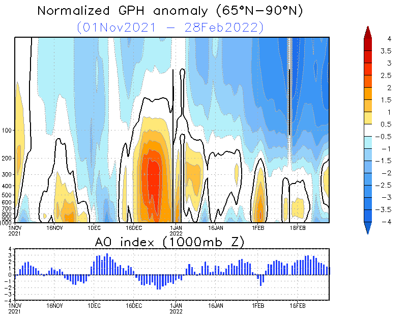
The daily geopotential height anomalies at 17 pressure levels are shown for the previous 120 days as indicated, and they are normalized by standard deviation using 1979-2000 base period. The anomalies are calculated by subtracting 1979-2000 daily climatology, and then averaged over the polar cap poleward of 65°N.
The blue (red) colors represent a strong (weak) polar vortex. The black solid lines show the zero anomalies.
The daily AO indices are shown for the previous 120 days, and the ensemble forecasts of the daily AO index at selected lead times are appended onto the time series. The indices are standardized by standard deviation of the observed monthly AO index from 1979-2000. A 3-day running mean is applied to the forecast time series.
The values at the upper left and right corners of each figure indicate the mean value of the AO index and the correlation coefficients between the observations and the forecasts, respectively.
The first panel shows the observed AO index (black line) plus forecasted AO indices from each of the 11 GFS ensemble members starting from the last day of the observations (red lines).
The ensemble mean forecasts of the AO index are obtained by averaging the 11 GFS ensemble members (blue lines), and the observed AO index (black line) is superimposed on each panel for comparison. For the forecasted indices (lower 3 panels), the yellow shading shows the ensemble mean plus and minus one standard deviation among the ensemble members, while the upper and lower red lines show the range of the forecasted indices, respectively.
From NCAR (for those with a more high-tech bend than I have:
The breakdown of the Stratospheric Polar Night Vortex is an atmospheric event that occurs once or twice each year in the polar wintertime stratosphere. As the polar vortex is formed, sharp gradients of potential vorticity at the vortex edge isolate polar air from the air at lower latitudes, producing conditions favorable for wintertime polar ozone depletion. Rossby waves propagating upward from the troposphere along the edge of the Polar Vortex grows exponentially in amplitude, eventually tearing the vortex apart.
The animations depict the flow of the Polar Vortex by visualizing Potential Vorticity (a variable that acts as a tracer) over the 16-day simulation. In the second and succeeding images, the height of the data has been greatly exaggerated to better show the rich vertical structure contained in the vortex. In reality, the vortex is only a few tens of kilometers thick, a pancake-thin region that can extend over much of the Northern Hemisphere.
This image shows a satellite view of the earth from space with three isosurfaces of Potential Vorticity mapped over the Northern Hemisphere from day 16 of the simulation. Brighter colors correspond to increasing Potential Vorticity. The animations at right, show the entire 16-day evolution
New radar technique locates storm-fueling water vapor
ScienceDaily, August 1, 2006 — People planning ball games, picnics, and other outdoor events may soon have more precise short-term forecasts of rainfall, thanks to an observing strategy now being tested by the National Center for Atmospheric Research (NCAR). An NCAR field project this summer is, for the first time, using multiple Doppler weather radars to track water vapor in the lower atmosphere. Measuring the low-level moisture is expected to help forecasters pin down the locations and timing of storms that might rage a few minutes to a few hours later.
The project is named REFRACTT (Refractivity Experiment For H2O Research And Collaborative operational Technology Transfer). Researchers are measuring changes in the speed of radar signals caused by refraction, which in turn reveal the presence or absence of atmospheric moisture. If the project proves successful, this refractivity technique could be added in the next few years to the national network of Doppler radars operated by NOAA's National Weather Service (NWS).
"Nobody's ever seen such high-resolution data on moisture before. We believe this could greatly help forecasters predict where heavy rains might develop," says NCAR scientist Rita Roberts, the lead principal investigator for REFRACTT.
REFRACTT runs from June 5 to August 11, 2006, and is being funded by the National Science Foundation, NCAR's primary sponsor. Along with four radars, scientists are using computer models, satellites, NCAR radionsondes (weather balloons), and ground-based sensors that intercept Global Positioning System signals and infer atmospheric moisture.
Strong contrasts in moisture can help to spawn intense storms, but the exact location of these contrasts is often hard to identify before storms develop. Currently, NWS radars detect rainfall and winds but not water vapor. Moreover, weather stations and weather-balloon launches that do measure water vapor are often separated by 50-100 miles or more. As a result, there is no regular monitoring of low-level moisture in between surface stations.
When meteorologists use Doppler radar to track storms, they normally monitor signals that strike raindrops, hailstones, or snowflakes and bounce back toward the radar. The strength of the returning signals indicates the intensity of rain, hail, or snow, while the change in signal frequency holds information on wind speed. During REFRACTT, scientists are adding a third variable: the speed of the radar signals. They are using fixed targets such as power lines and silos to see how much the radar signal is sped up or slowed down by variations in water vapor. The resulting data on refractivity is plotted on a map that shows scientists where the moisture is located.
The idea behind REFRACTT was developed by Frederic Fabry of McGill University while he was a visiting researcher at NCAR in the late 1990s. He has since collaborated with NCAR to refine the technique.
Forecasters at the Denver NWS office have been using REFRACTT data this summer to monitor the weather across northeast Colorado, including the risk of weak tornadoes that often spin up east of the Front Range. After the field project ends, the NWS will consider including refractivity as part of a larger upgrade to the national radar network.
"Low-level moisture is the key to our weather here, especially during the summertime," says Larry Mooney, meteorologist in charge at the Denver NWS office. "We're really excited about the REFRACTT data. I think it's a great example of how you can move technology into the operational realm pretty quickly if you're committed to it."
ScienceDaily, November 9, 2009 — The epic flooding that hit the Atlanta area in September was so extremely rare that, six weeks later this event has defied attempts to describe it. Scientists have reviewed the numbers and they are stunning.
"At some sites, the annual chance of a flood of this magnitude was so significantly less than 1 in 500 that, given the relatively short length of stream-gauging records (well less than 100 years), the U.S. Geological Survey cannot accurately characterize the probability due to its extreme rarity," said Robert Holmes, USGS National Flood Program Coordinator. "Nationwide, given that our oldest stream gauging records span about 100 years, the USGS does not cite probabilities for floods that are beyond a 0.2 percent (500-year) flood."
"If a 0.2% (500-year) flood was a cup of coffee, this one brewed a full pot," said Brian McCallum, Assistant Director for the USGS Georgia Water Science Center in Atlanta. "This flood overtopped 20 USGS stream gauges -- one by 12 feet. The closest numbers we have seen like these in Georgia were from Tropical Storm Alberto in 1994. This flood was off the charts."
The rains returned water levels in the region's two largest reservoirs, Lake Lanier and Allatoona Lake, to pre-drought levels. Lake Lanier rose by more than 3 feet to 1,068 feet by Sept. 25, 2009, and returned to full pool in October. Allatoona Lake rose to 853.25 feet on Sept 23, more than 13 feet over full pool of 840 feet.
"The flooding in Atlanta is certainly near the top of the list of the worst floods in the United States during the past 100 years," said Holmes. "For comparable drainage areas, the magnitude of this flood was worse than the 1977 Kansas City flood, which caused tremendous destruction and loss of life. It is a testament to the diligence of county officials and emergency management teams that more lives were not lost in Georgia."
Significant property losses, however, were a near certainty from this event. According to the National Weather Service, some locations recorded up to 20 inches of rain from 8:00 p.m. on Sept. 20, 2009, to 8:00 p.m. the following day. Culverts and sewers are not usually designed for events of this magnitude because they are so rare and the cost is prohibitive.
"Applying rainfall frequency calculations, we have determined that the chance of 10 inches or more occurring at any given point are less than one hundredth of one percent," said Kent Frantz, Senior Service Hydrologist for the National Weather Service at Peachtree City. "This means that the chance of an event like this occurring is 1 in 10,000."
For this analysis, USGS reviewed high-water-mark surveys and indirect peak discharge computations throughout the flood-affected region. Scientists gather these data from the field during floods and in their immediate aftermath to supplement or in this case, to provide data after a gauge is destroyed. Some notable results:
In Cobb County, Sweetwater, Noonday, Butler, and Powder Springs creeks flooded so severely that the annual chance of a worse event is far smaller than 0.2% (500-year) flood. On Sweetwater Creek near Austell, Ga., high-water marks showed a peak stage of 30.8 feet. The peak flow (31,500 cubic feet per second) was more than double the previous peak flow recorded at this site during the last 73 years. The previous peak, caused by the remnants of Hurricane Dennis in July 2005, was almost 10 feet lower at 21.87 feet.
In Douglas County, the Dog River near Fairplay overtopped the USGS stream gauge by 12 feet. The peak stage was 33.8 feet, with a peak discharge of 59,900 cubic feet per second. This is well beyond the 0.2% annual probability of exceeding a 500-year flood.
Gwinnett, DeKalb and Rockdale counties also had record flooding. Suwanee Creek floods were beyond the 0.2% annual probability of exceeding a 500-year flood.
On the Chattahoochee, the USGS gauge at Vinings reached a peak stage of 28.12 feet with 40,900 cubic feet per second, which represents between a between a 1.0 to 0.5% annual probability of exceeding a 100- to 200-year flood.
In Georgia, the USGS maintains a network of nearly 300 stream gauges that provide data in real time. Data from these stream gauges are used by local, state and federal officials for numerous purposes, including public safety and flood forecasting by the National Weather Service.
Geophysical Research Letters, 36 (2009) L20708; doi: 10.1029/2009GL040938.
Global surface cooling: The atmospheric fast feedback response to a collapse of the thermohaline circulation
Global surface cooling: The atmospheric fast feedback response to a collapse of the thermohaline circulation
A. Laurian, S. S. Drijfhout, W. Hazeleger and R. van Dorland (Royal Netherlands Meteorological Institute, De Bilt, Netherlands)
Received 10 September 2009; accepted 24 September 2009; published 28 October 2009.
Abstract
In the ECHAM5/MPI-OM model a collapse of the Atlantic thermohaline circulation results in a global surface cooling of 0.72 K. The mechanisms that are responsible for this cooling are investigated. Additional experiments were performed with a one-dimensional radiative convective model in which anomalies from the climate model were prescribed. Fast atmospheric feedbacks are essential to maintain and strengthen the global surface cooling caused by a THC collapse. Reduced downward long wave radiation exceeds the decreased upward long wave radiation. This decreased downward long wave radiation is caused by reduced water vapor content rather than by ice-albedo feedbacks. Also, the decrease in water vapor is much stronger than suggested by the water vapor feedback expected from the simulated albedo change. The large decrease in water vapor is the main feedback. On the regional scale, changes in cloud water and cloud radiative forcing further modify the surface cooling.
Nuuk Climate Days 2009: Changes of the Greenland Cryosphere Workshop & The Arctic Freshwater Budget International Symposium, Nuuk, Greenland, 25-27 August 2009
Primary author: DELTHLOFF, Klaus (Alfred Wegener Institute for Polar and Marine Research (AWI), Germany), Klaus.Dethloff@awi.de. Co-authors: RINKE, A. (Alfred Wegener Institute for Polar and Marine Research); HANDORF, D. (Alfred Wegener Institute for Polar and Marine Research); DORN, W. (Alfred Wegener Institute for Polar and Marine Research); BRAND, S. (Alfred Wegener Institute for Polar and Marine Research); MIELKE, M. (Alfred Wegener Institute for Polar and Marine Research); GRAESER, J (Alfred Wegener Institute for Polar and Marine Research); HERBER, A. (Alfred Wegener Institute for Polar and Marine Research)
Abstract ID: F1 The climate system of the Earth from a polar perspective
Balloon and radio sounding data from the North Pole drifting station NP35 for autumn 2007 to spring 2008 have been used to evaluate numerical model outputs (simulations with the regional climate model HIRHAM, ECMWF analyses). HIRHAM in the climate mode has some difficulty to represent the observed complex temperature profile, while the forecast mode shows better agreement. Sensitivity experiments concerning the atmospheric initial state, sea ice thickness and planetary boundary layer parameterization demonstrate improvements in the simulations.
Similar measurements have been carried out during spring 2009 on NP 36 and with the AWI airplane POLAR 5 over the Arctic Ocean. The pilot-project PAM-RCM (Pan-Arctic Measurements and Arctic Regional climate model simulations) provided a unique opportunity to obtain a snapshot of aerosol and cloud distributions and associated meteorological and atmospheric conditions as well as measurements of sea ice thickness in a latitude band between about 70°N and 80°N.
Sensitivity experiments using a coupled regional atmosphere-ocean-ice model of the Arctic has been conducted in order to identify the requirements needed to reproduce observed sea-ice conditions and to address uncertainties in the description of Arctic processes. While more sophisticated schemes for the albedo, the treatment of lateral freezing and melting, and the snow cover have been successfully introduced into the model, the parameterization of clouds is an open issue.
The global influence of Arctic feedbacks connected with sea-ice albedo changes and stratospheric ozone changes have been investigated. The simulations show significant changes over the Arctic and the whole globe due to changes of planetary wave patterns, which trigger the Arctic Oscillation (AO) and influences the sea -ice cover.
The impact of an interactive stratospheric ozone chemistry on the tropospheric circulation has been studied on the basis of the atmosphere-ocean-sea ice general circulation model ECHO-GiSP. The results show a sensitivity of the tropospheric circulation dynamics to the stratospheric chemistry. With enabled interactive stratospheric chemistry the model tends to the negative phase of the AO mode and a more unstable polar vortex..
Contact for symposium information: Sune Nordentoft Lauritsen, e-mail: snl@space.dtu.dk
Proceedings of the National Academy of Sciences, published online before print August 19, 2009; doi: 10.1073/pnas.0907610106
The physical basis for increases in precipitation extremes in simulations of 21st-century climate change
Paul A. O'Gorman* (Massachusetts Institute of Technology, Cambridge, MA 02139, U.S.A.) and Tapio Schneider (California Institute of Technology, Pasadena, CA 91125, U.S.A.)
Communicated by Kerry A. Emanuel, Massachusetts Institute of Technology, Cambridge, MA; July 14, 2009 (received for review March 24, 2009).
Abstract
Global warming is expected to lead to a large increase in atmospheric water vapor content and to changes in the hydrological cycle, which include an intensification of precipitation extremes. The intensity of precipitation extremes is widely held to increase proportionately to the increase in atmospheric water vapor content. Here, we show that this is not the case in 21st-century climate change scenarios simulated with climate models. In the tropics, precipitation extremes are not simulated reliably and do not change consistently among climate models; in the extratropics, they consistently increase more slowly than atmospheric water vapor content. We give a physical basis for how precipitation extremes change with climate and show that their changes depend on changes in the moist-adiabatic temperature lapse rate, in the upward velocity, and in the temperature when precipitation extremes occur. For the tropics, the theory suggests that improving the simulation of upward velocities in climate models is essential for improving predictions of precipitation extremes; for the extratropics, agreement with theory and the consistency among climate models increase confidence in the robustness of predictions of precipitation extremes under climate change.
aProgram for Climate Model Diagnosis and Intercomparison, Lawrence Livermore National Laboratory, Livermore, CA 94550;
bScripps Institution of Oceanography, La Jolla, CA 92037;
cNational Center for Atmospheric Research, Boulder, CO 80307;
dRemote Sensing Systems, Santa Rosa, CA 95401;
eInstitut für Unternehmensforschung, Universität Hamburg, 20146 Hamburg, Germany;
fCanadian Centre for Climate Modelling and Analysis, University of Victoria, Victoria, BC, Canada V8W 3V6;
gChemical Sciences Division, National Oceanic and Atmospheric Administration Earth System Research Laboratory, Boulder, CO 80305;
hHadley Centre, U.K. Meteorological Office, Exeter EX1 3PB, United Kingdom; and
iLawrence Berkeley National Laboratory, Berkeley, CA 94720
Abstract
In a recent multimodel detection and attribution (D&A) study using the pooled results from 22 different climate models, the simulated “fingerprint” pattern of anthropogenically caused changes in water vapor was identifiable with high statistical confidence in satellite data. Each model received equal weight in the D&A analysis, despite large differences in the skill with which they simulate key aspects of observed climate. Here, we examine whether water vapor D&A results are sensitive to model quality. The “top 10” and “bottom 10” models are selected with three different sets of skill measures and two different ranking approaches. The entire D&A analysis is then repeated with each of these different sets of more or less skillful models. Our performance metrics include the ability to simulate the mean state, the annual cycle, and the variability associated with El Niño. We find that estimates of an anthropogenic water vapor fingerprint are insensitive to current model uncertainties, and are governed by basic physical processes that are well-represented in climate models. Because the fingerprint is both robust to current model uncertainties and dissimilar to the dominant noise patterns, our ability to identify an anthropogenic influence on observed multidecadal changes in water vapor is not affected by “screening” based on model quality.
Study examines feedback mechanism that may be hastening Greenland ice-sheet melt
environmentalresearchweb.org, July 27, 2009
The Greenland ice sheet and the surrounding Arctic sea ice have experienced record levels of melting in recent years. But are the two linked? When sea ice melts does it encourage the ice sheet to melt too? A new study suggests that the answer to this question may be yes.
Satellite measurements show that the area of the Greenland ice sheet that experiences melting has increased by around 16% over the last 30 years. Meanwhile, Arctic sea-ice extent shrunk to a record minimum in the summer of 2007; 39% less than the long-term average. The years of 2008 and 2005 were also extreme; on average the summer sea-ice extent has been decreasing at more than 10% per decade for the last 30 years.
Climate models indicate that melting of the Greenland ice sheet is likely to increase global sea level by around half a metre over the next 100 years or so. But there is a large degree of uncertainty in this estimate, as there may be feedback mechanisms that could speed or slow the melting process.
Asa Rennermalm from the University of California in Los Angeles, and her colleagues have been investigating one potential feedback mechanism that may be hastening ice-sheet melt. Using satellite data gathered over the last 30 years, they looked at the way that the Greenland ice sheet and surrounding sea ice have changed in size over time.
They found a strong covariance between sea-ice extent and Greenland ice-sheet melt, particularly in the late summer of each year. The smaller the sea ice extent, the greater the rate of melting of the ice sheet. "They appear to work in concert," Rennermalm told environmentalresearchweb.
Not all regions of the ice sheet showed this covariance, but where it did occur – in the west and the southwest – it was very strong.
"We think that the presence or absence of sea ice may be influencing the surface climate over the ocean," said Rennermalm. Sea ice tends to cool and dry the air above it, whereas open-ocean is associated with warmer and wetter air. "With a favourable wind direction the lack of ice could act as an agent for bringing warm air to the ice sheet, increasing the rate of melting," she explained.
Right now all eyes are on the Jakobshavn ice-stream in Western Greenland, which lies just north of the current area of maximum melting – the Kangerlussuaq region. Models suggest that sea-ice retreat is going to march northwards. If so, the Jakobshavn ice-stream should be the next region to be hit. "It is a sweet spot for detecting the link," said Rennermalm.
The findings are published in Environmental Research Letters.
About the author
Kate Ravilious is a contributing editor to environmentalresearchweb.
Comment on ‘‘Climate forcing by the volcanic eruption of Mount Pinatubo’’ by David H. Douglass and Robert S. Knox
Alan Robock (Department of Environmental Sciences, Rutgers University, New Brunswick, NJ, U.S.A.)
Received 20 April 2005; accepted 27 July 2005; published 25 October 2005.
Citation: Robock, A. (2005), Comment on ‘‘Climate forcing by the volcanic eruption of Mount Pinatubo’’ by David H. Douglass and Robert S. Knox, Geophys. Res. Lett., 32, L20711, doi:10.1029/2005GL023287.
[1] Douglass and Knox [2005, hereinafter referred to as DK] present a confusing and erroneous description of limate feedbacks and the climate response to the 1991 Mt. Pinatubo eruption. Their conclusions of a negative climate feedback and small climate sensitivity to volcanic forcing are not supported by their arguments or the observational evidence. As pointed out by Wigley et al. [2005a], this is the consequence of assuming a one-box representation for the climate system, and ignoring energy exchange with the deep ocean.
[2] In the description of their analysis, DK make a fundamental mistake in describing the problem. They claim to use ‘‘standard linear response theory,’’ but they confuse the response with the forcing. They say, ‘‘The LW [longwave] effect is by definition the forcing function DF for the climate, represented by the measured surface temperature anomaly DT.’’ LW radiation changes, however, are produced by both the presence of a forcing agent, in this case stratospheric aerosols, and the response of the climate system. It is the instantaneous net radiation change with no response that is the forcing. The temperature anomaly is the response to forcing, and not the forcing itself, and the LW changes reflect both the true forcing and the effects of the temperature response.
[3] In spite of their statement to the contrary, DK apparently do use the correct forcing, as characterized by their equation (5) and illustrated in their Figure 2. Confusion arises because the forcing they use is a scaled version of the estimated aerosol optical depth changes, which represents the true forcing, yet they continually refer to the scaled optical depth as the LW changes. That the two items are different is clear from DK’s Figure 1.
[4] The forcing of climate change can be defined as the change in the net radiation at the top of the atmosphere, the tropopause, or the surface, without any response of the climate system, or allowing for the stratosphere to equilibrate. Stenchikov and Robock [1995], Houghton et al. [1996], and Hansen et al. [2005] discuss the standard definitions of radiative forcing and considerations for forcing from aerosols, which are not uniformly mixed in the atmosphere. For our purposes, it is sufficient to consider the forcing at the top of the atmosphere, allowing for no equilibration [Stenchikov & Robock, 1995; Stenchikov et al., 1998]. This forcing can be defined as:
(see link for the equations)
where DQ(t) is the radiative forcing, DSW(t) is the change in net downward shortwave radiation and DLW(t) is the change in net downward longwave radiation. Minnis et al. [1993] provide observations of changes in SW and LW separately after the 1991 Mt. Pinatubo eruption, but, of course, these observations combine the effects of forcing and response. Nevertheless, the SW changes are the largest, by an order of magnitude, and dominate the forcing. One cannot do a correct analysis if SW changes are ignored.
[5] Consider a global-average, time-dependent, anomaly energy-balance climate model:
(see link for equation)
where C is the heat capacity, DT(t) is the change in global temperature, l is the climate sensitivity (l = dT dQ), and DQ(t) is the externally applied radiative perturbation. (Much of the climate literature uses l1 or S as the climate sensitivity, but here the same nomenclature as DK is used to avoid confusion.) For a step-function forcing, at steady state the first term in (2) goes to zero and the final temperature change is:
(see link to pdf file for equation)
If DQ is due to a doubling of CO2, then DT is called DT2x. It is now conventional to characterize l in units of DT2x. The e-folding time scale of climate response is t (t = Cl). The amplitude of the climate response and the time it takes to respond to an episodic forcing are both dependent on DT2x.
[6] The value of l proposed by DK, 0.15 K/(W m2), corresponds to an unrealistic value of DT2x of 0.6 K. There is no evidence in the record of past climate change or in climate model simulations that the climate sensitivity could be so low.
[7] Soden et al. [2002] conducted general circulation model (GCM) simulations with the Geophysical Fluid Dynamics Laboratory Manabe climate model, forced by the observed distribution of Pinatubo aerosols. When run with prescribed clouds, their climate model, which has a DT2x 3.0 K, accurately reproduced not only the observed surface air temperature, but also the observed upper tropospheric humidity changes (consistent with a positive water vapor feedback), and the observed top of atmospherechanges in both SW and LW. To investigate feedbacks further, Soden et al. used two different versions of the model with explicitly modified sensitivity: the standard configuration, and a configuration with no water vapor feedback. Both GCMs had the same mixed-layer ocean heat capacity and were driven with the same forcing. The integrated cooling in the ‘‘no water vapor feedback’’ configuration was only 60% of that from the model with water vapor feedback. This is consistent with what one would expect for a gain factor of 0.4 from water vapor feedback (which is the expected value under the assumption of constant relative humidity), i.e., lðwith water vaporÞ ¼ lðno water vaporÞ ð1 0:4Þ: ð4Þ
Because they were able to observe each component of the feedback process, including the reduction of upper tropospheric water vapor with the Pinatubo-induced global cooling (a positive water vapor feedback), the Soden et al. study correctly showed how the Pinatubo eruption can be used to diagnose the sensitivity of the climate system and demonstrated that the sensitivity was in the conventional range.
[8] Wigley et al. [2005b], using a very different approach, obtained the same result as Soden et al. [2002]. They clearly showed that for episodic forcing, the transient temperature response of the climate system depends on C and DT2x, as characterized by both the maximum temperature change (DTmax) and the time scale of the response. (The response time in the Wigley et al. study is that for relaxation back to an equilibrium state, a time scale specific to volcanic forcing. It is called tV here, with the V used to indicate that it is specific to the volcanic forcing case. This time scale is not the same as the time scale that DK attempt to calculate, although they appear to think that it is.) Wigley et al. assigned to their MAGICC energy balance, upwelling diffusion climate model the same sensitivity as the National Center for Atmospheric Research PCM coupled ocean-atmosphere GCM. They found that, with this sensitivity, the MAGICC volcano results accurately matched the GCM, giving both the correct time scale and amplitude of climate response to volcanic eruptions, confirming that MAGICC can be used to measure the sensitivity of the climate system.
[9] Wigley et al. [2005b] then compared the results of MAGICC simulations with different sensitivities to the observed climate response after different eruptions. They found that DTmax / (DT2x)0.20 and tV [months] = 30 (DT2x)0.23. This is in contrast to the results of Lindzen and Giannitsis [1998], whose climate model results are inconsistent with GCM results. Lindzen and Giannitsis had found that DTmax / (DT2x)0.37 and tV = 57 (DT2x)0.41 and they erroneously implied from this that DT2x was quite low. By analyzing the observed temperature changes in response to the 1963 Agung eruption and the 1991 Pinatubo eruption, and fitting the response to their MAGICC model, Wigley et al. found that DT2x = 2.8 K for the 1963 Agung eruption and DT2x = 3.0 K for Pinatubo, and that tV = 38 months for both cases.
[10] As shown by the above two climate model analyses, in which the time delay and inertia of the ocean areexplicitly accounted for in the model physics, we expect the climate system to have a DT2x of about 3.0 K and for the peak cooling response after Pinatubo to be about 30% of the equilibrium response. The sensitivity calculated by DK, l = 0.15 K/(W m2), corresponding to DT2x of 0.6 K, means that if we use the observed maximum forcing of about 3.0 W m2 [0.165 (DK, Figure 2) times A (18.5 W m2/K, the mean of the DK values, 16 to 21Wm2/K)], the actual DTmax of 0.45 K (DK, Figure 3) is exactly equal to the equilibrium climate response we can expect (l x forcing) if the forcing were maintained. This is clearly wrong. Their failure to properly account for the entire climate system has led them to derive a climate sensitivity and response time that are much too small.
[11] To summarize, if the analysis is done correctly, the 1991 Mt. Pinatubo eruption serves as a valid test of the response of the climate system to external forcing [Robock, 2003]. As also discussed by Kerr [2004], this test provides additional evidence that the sensitivity of the climate system to doubling CO2 (DT2x) is about 3 K and that the water vapor greenhouse feedback is positive and can be observed.
Observational and Model Evidence for Positive Low-Level Cloud Feedback
Amy C. Clement,1,*Robert Burgman,1and Joel R. Norris2
Abstract
Feedbacks involving low-level clouds remain a primary causeof uncertainty in global climate model projections. This issuewas addressed by examining changes in low-level clouds overthe Northeast Pacific in observations and climate models. Decadalfluctuations were identified in multiple, independent clouddata sets, and changes in cloud cover appeared to be linkedto changes in both local temperature structure and large-scalecirculation. This observational analysis further indicated thatclouds act as a positive feedback in this region on decadaltime scales. The observed relationships between cloud coverand regional meteorological conditions provide a more completeway of testing the realism of the cloud simulation in current-generationclimate models. The only model that passed this test simulateda reduction in cloud cover over much of the Pacific when greenhousegases were increased, providing modeling evidence for a positivelow-level cloud feedback.
1 Rosenstiel School of Marine and Atmospheric Sciences, University of Miami, Division of Meteorology and Physical Oceanography, MSC 362, 4600 Rickenbacker Causeway, Miami, FL 33149, U.S.A. 2 Scripps Institution of Oceanography, University of California-San Diego, La Jolla, CA 92093–0224, U.S.A.
Clouds Appear to Be Big, Bad Player in Global Warming
Richard A. Kerr
The first reliable analysis of cloud behavior over past decades suggests—but falls short of proving—that clouds are strongly amplifying global warming. If that's true, then almost all climate models have got it wrong. On page 460, climate researchers consider the two best, long-term records of cloud behavior over a rectangle of ocean that nearly spans the subtropics between Hawaii and Mexico. In a warming episode that started around 1976, ship-based data showed that cloud cover—especially low-altitude cloud layers—decreased in the study area as ocean temperatures rose and atmospheric pressure fell. One interpretation, the researchers say, is that the warming ocean was transferring heat to the overlying atmosphere, thinning out the low-lying clouds to let in more sunlight that further warmed the ocean. That's a positive or amplifying feedback. During a cooling event in the late 1990s, both data sets recorded just the opposite changes—exactly what would happen if the same amplifying process were operating in reverse.
Add CO2 to the atmosphere and the climate will get warmer — that much is well established. But climate change and carbon aren't in a one-to-one relationship. If they were, climate modeling would be a cinch. How much the globe will warm if we put a certain amount of CO2 into the air depends on the sensitivity of the climate. How vulnerable is the polar sea ice; how rapidly might the Amazon dry up; how fast could the Greenland ice cap disintegrate? That's why models like those from the Intergovernmental Panel on Climate Change spit out a range of predictions for future warming, rather than a single neat number.
One of the biggest questions in climate sensitivity has been the role of low-level cloud cover. Low-altitude clouds reflect some of the sun's radiation back into the atmosphere, cooling the earth. It's not yet known whether global warming will dissipate clouds, which would effectively speed up the process of climate change, or increase cloud cover, which would slow it down. (See pictures of the effects of global warming.)
But a new study published in the July 24 issue of Science is clearing the haze. A group of researchers from the University of Miami and the Scripps Institute of Oceanography studied cloud data of the northeast Pacific Ocean — both from satellites and from the human eye — over the past 50 years and combined that with climate models. They found that low-level clouds tend to dissipate as the ocean warms — which means a warmer world could well have less cloud cover. "That would create positive feedback, a reinforcing cycle that continues to warm the climate," says Amy Clement, a climate scientist at the University of Miami and the lead author of the Science study.
Getting data on cloud cover isn't easy. There is reliable information from satellites, but those only go back a few decades — not long enough to provide a reliable forecast for the future. Clement and her colleagues combined recent satellite data with human observations — literally, from sailors scanning the sky — that go back to 1952, and found the two sets were surprisingly in sync. "It's pretty remarkable," says Clement. "We were almost shocked by the degree of concordance."
The data showed that as the Pacific Ocean has warmed over the past several decades — part of the gradual process of global warming — low-level cloud cover has lessened. That might be due to the fact that as the earth's surface warms, the atmosphere becomes more unstable and draws up water vapor from low altitudes to form deep clouds high in the sky. (Those types of high-altitude clouds don't have the same cooling effect.) The Science study also found that as the oceans warmed, the trade winds — the easterly surface winds that blow near the equator — weakened, which further dissipated the low clouds.
The question now is whether this process will continue in the future, as the world keeps warming. Scientists create climate models to try to predict how the earth will respond to higher levels of greenhouse-gas emissions, but only one model — created by the Hadley Centre in Britain — includes the possible impact of changing cloud behavior. And the bad news is that the Hadley model contains particularly high temperature increases for the 21st century, in part because it sees dissipating cloud cover as a positive-feedback cycle — meaning the warmer it gets, the less cloud cover there will be, which will further warm the earth. Though it's just one data set over one part of the earth's surface, the Science study indicates that the pessimistic Hadley model may be right. "These low clouds are like the mirrors of the climate system," says Clement. "If they disappear, you might see that positive-feedback cycle." (See the top 10 green ideas of 2008.)
Cloud cover is only one element of climate sensitivity. Scientists are also concerned about the earth's ice, which reflects sunlight back into space, making it a cooling factor, while seawater absorbs the sun's heat. That means that as polar sea ice melts because of warming, leaving more open water, the warming process could accelerate — which would then melt more ice. There are also concerns that as the permafrost in the Arctic thaws, it could release massive amounts of methane, a powerful greenhouse gas that would further accelerate warming.
And then there's the Amazon. Right now, the rain forest is a huge carbon sink, which compensates for the greenhouse gases we release by burning fossil fuels. But if the climate warms so much that the rain forest begins to die off — a distinct possibility — we'll lose that carbon sink, and then warming will again accelerate. Scientists, including the authors of the Science study, are still trying to nail down exactly where these tipping points might be — but it seems that the more we find out, the more the evidence points to an increasingly sensitive climate. And that's bad news for us.
Geophysical Research Letters, 35 (2008) L20704; doi:10.1029/2008GL035333
Water-vapor climate feedback inferred from climate fluctuations, 2003–2008
Water-vapor climate feedback inferred from climate fluctuations, 2003–2008
A. E. Dessler, Z. Zhang and P. Yang (Department of Atmospheric Sciences, Texas A&M University, College Station, TX, U.S.A.)
Abstract
Between 2003 and 2008, the global-average surface temperature of the Earth varied by 0.6°C. We analyze here the response of tropospheric water vapor to these variations. Height-resolved measurements of specific humidity (q) and relative humidity (RH) are obtained from NASA's satellite-borne Atmospheric Infrared Sounder (AIRS). Over most of the troposphere, q increased with increasing global-average surface temperature, although some regions showed the opposite response. RH increased in some regions and decreased in others, with the global average remaining nearly constant at most altitudes. The water-vapor feedback implied by these observations is strongly positive, with an average magnitude of λq = 2.04 W/m2/K, similar to that simulated by climate models. The magnitude is similar to that obtained if the atmosphere maintained constant RH everywhere.
(Received 13 July 2008, accepted 19 September 2008, published 23 October 2008.)
Dessler, A. E., Zhang, & P. Yang, P. (2008), Water-vapor climate feedback inferred from climate fluctuations, 2003–2008, Geophysical Research Letters, 35, L20704; doi:10.1029/2008GL035333.
There is a simple way to produce a perfect model of our climate that will predict the weather with 100% accuracy. First, start with a universe that is exactly like ours; then wait 13 billion years.
THE PHYSICS THAT WE KNOW [6.29.09] A Conversation with Gavin Schmidt
Introduction
There is a simple way to produce a perfect model of our climate that will predict the weather with 100% accuracy. First, start with a universe that is exactly like ours; then wait 13 billion years.
But if you want something useful right now, if you want to construct a means of taking the knowledge that we have and use it to predict future climate, you build computer simulations. Your models are messy, complicated, in constant need of fine tuning, exacting and inexact at the same time. You're using the past to predict the future, extrapolating the very complicated from the very simple, and relying on an ever-changing data stream to inform the outcome.
Climatologist Gavin Schmidt explains: "How do you ask questions about expectations in the future? Obviously, you have to have things that are based on the physics that we know. You have to have things that are based on processes we can go and measure, that has to be based on our ability to understand the climate that we have now. Why do you get seasonal cycles? Why do you get storms? What controls the frequency of these events over a winter, over a longer period? What controls the frequency of, say, El Nino events in the tropical Pacific that have impacts on rainfall in California or in Peru or in Indonesia? How do you understand all of those things?"
"We approach this is in a very ambitious way."
"What we have decided, as a scientific endeavor, is to extrapolate as much as we can from our knowledge of the individual processes that we can measure: evaporation from the ocean, the formation of a cloud, rainfall coming from a cloud, changes in the wind patterns as a function of the pressure field, changes in the jet stream. What we have tried to do is encapsulate those small-scale processes, put them altogether, and see if we can predict the emerging properties of that fundamental complex system."
— Russell Weinberger
GAVIN SCHMIDT is a climatologist with NASA's Goddard Institute for Space Studies in New York, where he models past, present, and future climate. GAVIN SCHMIDT is a climatologist with NASA's Goddard Institute for Space Studies in New York, where he models past, present, and future climate. His essay "Why Hasn't Specialization Led To The Balkanization Of Science?" in included in What's Next? Dispatches on the Future of Science, edited By Max Brockman
[GAVIN SCHMIDT:] In terms of environmental problems, the key question that faces us now (and will face us for at least the next century) is to what extent are the changes that we are making to the atmosphere — to the oceans, to the composition of the air — going to impact things that matter? How are they going to impact sea level changes? How they are going to impact temperature changes? How they are going to impact rainfall and hydrological resources?
Everywhere you go you see societies based around certain expectations for what their climate is. How far do you build away from the shore? How do you design your agriculture? What kind of air conditioning system do you put in a building? All of these things depend on the expectations you have for what temperature it is going to be during the summer time or how high a storm surge reaches when you have a Northeasterly storm. All of these things require an expectation that has been built over hundreds of years but that now is changing.
When you have expectations based on past information that aren't any longer going to be valid expectations or you have a suspicion that they are no longer going to be valid, how do you come up with new expectations? How do you inform decisions that are being made now that will affect how people react to climate in 10, 20, 30, 50 years time? We are building infrastructure now that has those kinds of lifetimes and yet are we using our best estimate of what is going to happen in the future to inform those decisions? The answer is pretty much no. We know that is not being done.
So, how do you ask questions about expectations in the future? Obviously, you have to have things that are based on the physics that we know. You have to have things that are based on processes we can go and measure, that has to be based on our ability to understand the climate that we have now. Why do you get seasonal cycles? Why do you get storms? What controls the frequency of these events over a winter, over a longer period? What controls the frequency of, say, El Nino events in the tropical Pacific that have impacts on rainfall in California or in Peru or in Indonesia? How do you understand all of those things?
We approach this is in a very ambitious way.
What we have decided, as a scientific endeavor, is to extrapolate as much as we can from our knowledge of the individual processes that we can measure: evaporation from the ocean, the formation of a cloud, rainfall coming from a cloud, changes in the wind patterns as a function of the pressure field, changes in the jet stream. What we have tried to do is encapsulate those small-scale processes, put them altogether, and see if we can predict the emerging properties of that fundamental complex system.
This a very ambitious thing to attempt to do because there is a lot of complexity, a lot of structure in the climate that is not a priori predictable from any small scale process. The wet and dry seasons in the tropics come about because of the combination of the seasonal cycle of the orbit around the earth, changes in evaporation, changes in moist convection (the process that creates the big cumulus towers and thunderstorms), water vapor transports because of the moist convection, because of the Hadley Cell that gets set up as a function of all those things. It's a very complex environment. I can't say how it is going to change if evaporation was a little bit different or the sensitivity of evaporation was a little bit different to what we understand now.
We have been quite successful at building these models on the basis of small-scale processes to produce large-scale simulation of the emerging properties of the climate system. We understand why we have a seasonal cycle; we understand why we have storms in the mid latitudes; we understand what controls the ebb and flow of the seasonal sea ice distribution in the Arctic. We have good estimates for all the things that are going on. But we don't have perfect estimates. Instead, we have maybe 20 different groups around the world who have put together their best shot at what all those process are, which ones are important and which ones are not important, and they have all produced their own separate digital world, their digital climate. They are all a little bit different and they all have a little bit different sensitivity. So if I change one element in those models, for instance the amount of carbon dioxide in the atmosphere, then they all react in slightly different ways.
In some respects they all act in very similar ways — for instance, when you put in more carbon dioxide, which is a green house gas, it increases the opacity of the atmosphere and it warms up the surface. That is a universal feature of these models and it is universal because it is based on very, very fundamental physics that you don't actually need a climate model to work out. But when it comes to aspects which are slightly more relevant – I mean, nobody lives in the global mean atmosphere, nobody has the global mean temperature as an important part of their expectations – things change. When it comes to something like rainfall in the American Southwest or rainfall in the Sahel or the monsoon system in India, it turns out that those different assumptions that we made in building those models (the slightly different decisions about what was important and what wasn't important) have a very important effect on the sensitivity of very complex elements of the climate.
Some models suggest very strongly that the American Southwest will dry in a warming world; some models suggest that the Sahel will dry in a warming world. But other models suggest the exact opposite. Now, let's just imagine that the models have an equal pedigree in terms of the scientists who have worked on them and in terms of the papers that have been published — it's not quite true but it's a good working assumption. With these two models, you have two estimates — one says it's going to get wetter and one says it's going to get drier. What do you do? Is there anything that you can say at all? That is a really difficult question.
There are a couple of other issues that come up. It turns out that if you take the average of these 20 models, that average is a better model than any one of the 20 models. It has a better prediction of the seasonal cycle of rainfall; it has a better prediction of surface air temperatures; it has a better prediction of cloudiness. That is a little bit odd because these aren't random. You can't rely on the central limit theorem to demonstrate that that must be the case, because these aren't random samples. They are not 20 random samples of the space of all possible climate models. They have been tuned and they have been calibrated and they have been worked on for many years — everybody is trying to get the right answer.
In the same way that you can't make an average arithmetic be more correct than the correct arithmetic, it's not obvious that the average climate model should be better than all of the other climate models. So for example if I wanted to know what 2+2 was and I just picked a set of random numbers, the answer by averaging all those random numbers is unlikely to be four. Yet when you come to climate models, that is kind of what you get. You get all the climate models and they give you some numbers between three and five and they give you something that is very close to four. Obviously, it's not pure mathematics — it's physics, it's approximations, there is empirical tuning that goes on. But it's very odd that the average of all the models is better than any individual model.
Does that mean that the average of all the models predictions is better than any individual model's prediction? That doesn't follow either because it may be that all the models contain errors which, for today's climate, average out when you bring them together. Who is the say what controls their sensitivity since we know that, in each model the sensitivity is being controlled by slightly different elements?
You need to have some kind of evaluation. I don't like to use the word validation because it implies a kind of binary/true-false set up. But you need an evaluation; you need tests of the model's sensitivity compared to something in the real world that can give you some credibility that that model has the right sensitivity. That is very difficult. For instance, let's imagine that the models that I want to pay attention to are the ones that get the best seasonal cycle of rainfall. So I rank the models, give them a score, and I get the top 10 models that come in with the best score for that metric. Then somebody else says, no, I think it's more important that they get the annual mean right or they get the inter-annual variability — the variability from one year to another. Well, I could do that same ranking. It turns out that if I do that ranking for three different metrics — there is nothing that says that one metric is better than the other — I end up with 10 completely different rankings. Not only are the rankings uncorrelated one from to the other, depending on the metric, the projections — the estimates that you get going into the future — turn out to be uncorrelated to the score as well. I get the same spread if I take the top 10 models over here than I had for the whole set. So there will still be some positive ones, there will still be some negative ones when it I look, for instance, at projected rainfall in the American Southwest.
That is a real problem. How do you deal with these models in an intelligent way? What can you bring to bear from the observational record where either over the 20th century or longer (paleo-climate records or what have you)? how do you bring that information to bear to test whether the models have any predictable skill, have any skill in their predications? That is really what I spent all my time on: trying to find ways to constrain the models to improve the Bayesian subjective probability that they are telling you anything of any use. It's not that we have been working in a complete vacuum for the last 30 years. These models are relatively mature and people have been thinking about these things ever since the beginning.
There are lots of examples in the current climate where you can demonstrate that the models have skill. The response to the Mount Pinatubo eruption in 1991. This was a big volcano in the Philippines. It put a huge amount of sulphur dioxide and sulphur aerosols into the atmosphere. They spread around the stratosphere, stayed there for about two to three years. These aerosols are reflective; they are white. So the sun comes in, there are these aerosols, it gets reflected out. It acted as a kind of sun shade over the planet and it caused the planet to cool. Our group (though this is before my time) before this cooling happened, did the calculations with their model at the time, and said, that the cooling will reach a maximum of about half a degree in about two years time. Lo and behold, such a thing happened. If you go back – and we had lots and lots of information about what happened over that period, what happened to radiation at the top of the atmosphere, what happened to the winds that changes the function of the temperature gradients in the lower stratosphere, what happened to water vapor – we can see whether the models got the right answer for the right reason, and for the most part they do. So that was a good real prediction in real time that could be tested in a short amount of time.
The problem with climate prediction and projections going out to 2030 and 2050 is that we don't anticipate that they can be tested in the way you can test a weather forecast. It takes about 20 years to evaluate because there is so much unforced variability in the system which we can't predict — the chaotic component of the climate system — which is not predictable beyond two weeks, even theoretically. That is something that we can't really get a handle on. We can only look at the climate problem once we have had a long enough time for that chaotic noise to be washed out, so that we can see that there is a full signal that is significantly larger than the inter-annual or the interdecadal variability. That is a real problem because society has demanded answers of us and isn't going to wait 20 years for us to update.
We did this 20 years ago and the predictions that we made then have been more or less validated, given both the imperfections that we had then and the uncertainty in how we thought things were going to change in the future. So there is a track record that shows that these models are realistic. But the questions that were asked 20 years ago were relatively simple compared to the questions that are being asked now. The issue of climate change has become so tied into many other questions, such as biosphere degradation, habitat loss, over-development, inappropriate development, energy security, etc.. All of these questions are much more immediate and acute than climate change as a whole. Yet climate change impacts very strongly on how you might deal with a lot of those issues. Society is not willing just to wait for the scientists to say "come back in 20 years and we will tell you whether our predictions are any good or not." It's tricky. People want answers and the need to validate those answers but we have to do it in a way that is not the standard: make a prediction, test it; make a prediction, test it. The time scales are just too long.
The thing that you have with climate and really with any observational science, as opposed to a laboratory science, is that you have history. Essentially you have 4.5 billion years of earth history, of which we know increasingly little the further you go back. But we do know a fair bit about how climate has changed in the past. We know about the ice ages 20 thousand years ago. We know about oscillations in the ocean circulation that happened around 8,000 years ago. We know that 6,000 years ago the Sahara was much wetter than it is now. We have theories for why all of those things happened based on our knowledge of planetary dynamics, how the orbit has changed in that time period, how the de-glaciation (the melting of the big ice sheets from about 20,000 years ago to about 8,000 years ago) proceeded. We have clues about that in ice core records, in the continual uplift of where the ice sheets used to be, in drainage pathways of the paleo great lakes that existed at that time. We can see where the beaches were. There are a lot of clues in the landscape, in the geology, in the soils, in the sea, in the mud, in the ice, in tree rings, in corals that give us clues about how things changed in the past. But all of those clues are very indirect. They're not real thermometers. They're not rain gauges. They're not satellites. They are telling us things that are connected to climate but are not really the same as climate. Interpreting them has always been problematic because they are often a function of, not one particular thing that is changing the climate, but maybe four or five different things, all of which are changing in different ways at different times.
Over the last five years or so we have spent an enormous amount of effort making the climate models that we use much more complete. It used to be that we would have basically the atomospheric circulation and the water cycle — those are the key elements to the climate system. But there is a lot more going on. There is mineral dust. There are aerosols and these aerosols interact with the clouds, they interact with radiation, they have interactions with atmospheric chemistry, they have interactions with air pollution and other kinds of emissions to produce ozone (also a greenhouse gas, but it is something that is generated within the atmosphere rather than being emitted as a pollutant). Those aerosols and those other elements of atmospheric composition make the whole problem much more complicated and they add huge numbers of extra pathways that allow temperature changes or hydrological cycle changes or wind changes to intersect with greenhouse gases and temperatures and the like.
The neat thing is that these same chemicals are also very closely related to the things we measure in ice cores and in mud in the bottom of the ocean. We can measure dust records in the ice cores, which tell us how much dust got to Greenland pretty much every year for the last 100,000 years. That is telling us something about where that dust was coming from. It tells us something about the atmospheric circulation, but it's one variable that depends on many different inputs. But because we have now included that in the climate models, we can now ask questions like, "given this hypothesis for why the climate changed at that point, does the simulated dust record that we would have gotten in our numerical virtual Greenland match up to what we actually see in the real Greenland?" Then we can go back and look at the climate changes and the ideas that we have had for why the climate changed in the past and evaluate how well the models do with really large changes in climate. That is potentially much more useful than testing the models against the seasonal cycles today because you are testing against a real climate change as opposed to a proxy for climate change.
Things that happen over the seasons are very different than things that happen due to an increase carbon dioxide over time. They are a very different physically; the time scales are different; you have different kinds of feedbacks. But if you go back into the past, you can see those same long term feedback effects that control what is going to happen in the future, operating over a similar time period. The reason the Sahara was green 6,000 years ago is that we were a little bit closer to the sun during Northern Hemisphere summers because of the way the orbit of the earth works. We're on an ellipse and there is a point where we are close to the sun, there is a point where we are far away from the sun. Right now we are closest to the sun in January; 6,000 years ago we were closest to the sun in August. So August is Northern Hemisphere summer and you are going to get warmer summers. As you have warmer summers, that moves the thermal equator to the north, and the rain bands tend to follow that thermal equator, go much further into the Sahara than they would today. The models show that same sensitivity and that gives you some hope that these models are actually telling us something realistic.
The problem is that most of the modeling groups don't do those kinds of experiments. Right now we are in the midst of building a new huge database of model simulations that will be used for the next IPCC report. The IPCC (the Intergovernment Panel on Climate Change) is an assessment body which goes around looking at all the things that are in the scientific literature and coming up with an assessment what it all means. The community of climate modelers know that these things are coming up and what they do a few years beforehand is they put together a huge database of simulations that people can look at, so that by the time the IPCC comes along and says, "what is going on in the world of climate modeling?", there will be lots of information about all these different climate models. We are working to make sure that within these sets of simulations, people are running their models for paleo-climate simulations, so that we can do exactly what I was trying to allude to: can we rate the models based on how well they do in the paleo-climate? Does that give us an idea that models with low sensitivity are better for the future or is it going to be the ones with high sensitivity? We are going to have a metric that is much closer to what we think we need to make up some kind of assessment of how credible we think the projections are going to be.
Freeman Dyson has made a critique of models. I don't know Freeman Dyson; I've met his children. He seems like a very smart person. He has done some very interesting physics. He seems like a guy I would like to know. Yet his statements about climate, climate models, climate modelers, Jim Hansen in particular, are not the statements you would expect a smart person to make. It's like Shakespeare writing a play and then pulling a quote from a penny dreadful sheet that he found in the street. It just seems very inconsistent that somebody who thinks so hard and is so smart about so many things says dumb things like, oh, climate modelers think that their models are real and can't see the real world. I paraphrase but he said something very similar. It betrays a complete ignorance of either climate modelers, climate models or what it is that climate science is all about. His statements about Jim Hansen were very similar.
Jim Hansen (my boss, so take what I say with a pinch of salt if you prefer) is not anything like the caricature that Dyson painted, and anybody who says that has never met him, has never read anything that he has actually written, and is just responding to, I imagine, the kind of online simulacrum that you sometimes find with people who are high profile that actually bears no relation to their real ideas or personality or expertise. I'm much less famous than Jim Hansen but I sometimes see discussions about me and my opinions and my expertise that are just so far removed from anything that I would ever say or would ever think that it is laughable. Yet Dyson, who is a smart person, seems to be reading something like that, as opposed to investigating and talking to these people for himself. I find that puzzling.
Climate change is one of those scientific topics where people perceive that the science itself is imbued with some moral, political or economic meaning. Just like stem cell research or evolution of genetically modified food — people react very strongly to what they perceive the science implies, to the extent where they attack the science rather than discuss the issue of how that science implies something that is more fundamental. It turns out that in many of these fields, people are much more wedded to their moral, political, tribal viewpoints than they are to scientific method and scientific inquiry. This is not surprising, and it takes years to beat that into graduate students — it's not something that people are naturally going to come up with. Yet when you have great scientists who are able to imply their scientific thinking in many, many different fields, and when it comes to one particular issue seem to not be thinking as critically, it's a surprise. So statements like Freeman Dyson's or Will Happer's or Karry Mullis or Linus Pauling toward the end of his life, these are very smart people who have been lauded for being very smart their entire lives. Sometimes they say things that are very strange.
I understand that Dyson is a bit of a contrarian and that part I don't find bothersome in the slightest. Anybody who is a good scientist has to have that contrarian streak. They have to be the kind of person who says, "oh yeah? Prove it." You have to be that way. You can't just go around agreeing with everyone if you are going to make a contribution. You have to listen to everything that is going on. You see where the weak points are, you see where the assumptions are, and you burrow down into assumptions and you say, "is that really justified?" Quite often you find that it isn't. When it isn't justified and it has important consequences, then you have made a contribution as a scientist.
An example: I was talking about paleo-climate before. A lot of the interpretation of paleo-climate rests on very weak assumptions and my modest contributions to the field has been in tackling exactly those assumptions. So you have to have that contrarian streak. You have to have that questioning streak. That doesn't surprise me in the least that most good scientists have that attitude. But in the best scientists that attitude is also married with a humility — maybe you don't know everything that is going on. You can come into a field and say, "these people seem to be making this assumption, how have they analyzed it?" Generally speaking, they have analyzed it to death. When you come into a new field or when you comment on a field that isn't something that you have grown up with over time, you have to come in with a humility that says, these people are smart as well, and let me see how they have used their smarts. I didn't get that sense when Freeman Dyson was talking about climate change.
I started off with pure math, applied math, fluid mechanics, special relativity, that kind of stuff. What I saw as I went through my education was a very clear winnowing out — not between really smart people and not smart people — but between people who had an aesthetic sense for the kinds of problems that they found interesting and useful. The way that would work out is that those interested in theoretical physics were the people who enjoyed finding a problem that is amenable just to being thought at. This is not trivial. There aren't that many problems like that, but when you have that can be thought at you can come up with the key insight, then you have something that really changes the world. Einstein thinking about special relativity is a good example. So is QED. Those problems have an aesthetic quality to them that is very attractive: it's not messy, it's not horribly complex (general relativity and things that have come from it are very complex, of course, but they stem from relatively simple systems).
Then there the kinds of problems that attract a different kind of thinker: really, really complex problems, such as the human body or an individual cell or the climate system or solar physics. These are subjects that don't fit into the same aesthetic that special relatively fits into. They demand, right from the beginning, that you deal with multiple conflicting and intersecting elements. They are horribly non-linear right from the word go; they are horribly complex. There is never going to be a theory of climate that somebody is going to come up with just by thinking about how the climate should work. People have tried, but they all fall pretty much at the very first hurdle. It is, to use a phrase, irreducibly complex.
And you can't get away from that. You can't think that the climate is ever going to yield by just being thought about. It needs to be thought about and measured and analyzed and thought about again and measured and analyzed and all of these disparate elements have to brought in together. The reason why climate models have grown up to be as complicated and as complete as they are is not because of a lack of imagination from the people who are using them. It's because that is the way the real world is and that is the way the field has made progress. It hasn't made progress by people sitting in a room coming up with theories for how climate should work. It's made progress because people have made complex assumptions; they have built these things into models of varying complexity, all the way to the GCMs, (the big climate models that I was talking about earlier); they have been tested against very complex data from satellites, from intense observation campaigns, from In-situ observations. At the same time, all these models are plagued with uncertainty and have the problem of changing measurements. The data collecting is always improving and our understanding of different processes is always growing. But that doesn't make things simpler, it makes things more complex. It means you need to add another element to your model. It means you have to measure everything again and run the model again.
You have to be the kind of scientist who embraces complexity in order to make progress in this kind of field. There are a lot of scientists who do not have that approach to complexity, specific kinds of physicists who have self-selected themselves as the people who want to deal with aesthetically pleasing problems from their point of view. Climate change is not that kind of science.
Now, there are some very big questions that we face as climate scientists and some very specific problems that we need to approach. Let me give you an example of an analysis that I think will be very interesting.
Every individual storm in the mid-latitudes is different — each has a different shape, a different amount of rainfall, the clouds are different, etc. The ability of the climate model to reproduce exactly the same weather pattern that we have seen over time is just about zero. That is, trying to reproduce exactly what has happened in the right time sequence season by season, day by day, is something we are not going to be able to do.
But what we are interested in is what happens to the generic storm. There is enough similarity between one low-pressure system and another low-pressure system that if you put them all together, you would come up with a generic storm. It would have a lot of information that was common to all of those storms but not the information that was unique to any one storm that happened to be in one particular configuration.
There is a constellation of satellites called the A-Train that is run by NASA: five polar orbiting satellites, that fly in formation so that there is about a 20 minutes difference from the first one and the last one. They are flying in something like a train and they are all pointing pretty much the same point on the surface of the earth as they are traversing. They are measuring many, many different things: they are measuring the temperature of the atmosphere, how many aerosols there are, how much sea ice there is, the amount of chlorophyl in the ocean below, the winds at the surface, etc. etc. Every time they pass over they will see a little bit of a storm. They will pass over a storm and the next day they might pass over it again as it has shifted a little bit to the west.
Collectively, over the 7 or so years that these satellites have been up there, they have seen many, many different storms which very similar characteristics. Wouldn't it be great if you could just take that satellite data and then make that composite storm based on the weather models that tell us where the storms were? You would take a time-space map of weather models that tracked the storms in a given area and see when the satellites were passing over storms. Collect all of that data and you'd be able to come up with a statistically average storm for that area over that whole seven year period.
This would be a tremendously valuable tool that we could use to develop our models – to compare the ACTUAL average storm with the model's prediction. You would think that someone would do this study but nobody has. All of that satellite data is there (it's only a few petabytes), all of that model information is there. Why hasn't the study been done? The reason is each individual data stream for each of those different individual instruments on the satellites — even though they are all run by NASA — is in a different place. And the way that the time/space information has been collated for each of those instruments is different. There is no single portal that would allow you to filter that data without having to the entire data set to your hard drive and sorting it yourself. Of course you can't do that because it's petabytes of data and there is no hard drive that contains petabytes of data.
The same is true for the models: all the models come in the same kind of box, but if you want the temperatures, you have to download the entire grid of temperatures for every, for every month for the entire period. There is no intelligent filtering in-situ so, again, you have to download gigabytes and gigabytes of data in order to derive one small set of numbers. Even if your network connection would allow you to download that much information in any kind of reasonable time period.
So that is the sort of problem we face. Using the satellite data to see how well the models predict an average storm or the processes within it is a completely sensible thing to be doing. But it's completely impossible. It would take, I imagine, something like 100 man years to do it with the current data set as it is currently configured.
But this doesn't require a huge a leap in technology to solve. This is really just a processing problem. It's the kind of thing that falls in between the cracks because it's not interesting enough a research problem for a computer scientist to be interested in, but it's too large a task for a scientist to want to devote any time to. So you have this big grey area in between the cool research on networks/computer science/machine learning, and what is needed to approach very interesting scientific questions that is far too large for any one individual or group of scientists to put together themselves.
It's just not getting any attention and that is something, it seems to me, that is going to be a defining quality for the information-rich 21st century — that there is going to be a gap between what is needed by certain groups of people and what is ready to be supplied by the groups of people who are doing things that are much cooler. The question I am asking is, how do you fill that in? How do you get funding agencies to understand that this might be a little pedestrian but is absolutely fundamental?
Google had an initiative called Google Research Data Sets, where I spent a lot of time talking to people, giving them exactly this problem and challenging them to do something about it. They have the capacity. They have the know-how. It was a very interesting idea but, in the end, they canceled the whole project.
And this brings us to the question of "what do we do about it"? How should scientists get involved in policy. Lots of different scientists come to very different decisions about that. I think it's nice that different scientists come to different decisions and that there is a range of opinion about how strongly one should interact with the policy process.
Personally, I don't pretend to be an economist; I don't pretend to be a sociologist; I don't pretend to be an expert in environmental regulation. So I generally don't comment on whether a cap and trade system is better than a carbon tax system or whether or not it is better that it is being run by the EPA. I leave that kind of stuff for the people who focus on that much more specifically, and I'm pretty much willing to find the most interesting and objective of them and give them the benefit of the doubt.
It's clear that there are a lot of people who talk about politics who are neither interesting nor objective. When it comes to discussing what to do about climate change, it appears to be a fact of life that people will use the worst and least intelligent arguments to make political points. If they can do that by sounding pseudoscientific — by quoting a paper here or misrepresenting another scientist's work over there — then they will. That surprised me before I really looked into it. It no longer surprises me.
I don't advocate for political solutions. If I do advocate for something, (and if you put your voice into the public sphere, then it has to be to advocate for something. Why would you do it otherwise?) My advocacy is much more towards having more intelligent discussions, which is completely naive and stupid and I realize that.
Five years ago I was less of a public person — less of a public persona in climate-science than I am now. But at the time, the voices that were being heard discussing climate change were completely divorced from the actuality of what people were coming through with the science. The Wall Street Journal was featuring full-on attacks on scientists; congress was filled with know-nothings; and, in the mainstream media, every time there was a story, you would have to one of the five obligatory contrarians pop up and say "oh no, everything is going to be fine."
It was just distortion upon distortion, and there was no advocacy from the community that was actually studying this. There was no public voice for the community. There were a few scientists who would step out occasionally — Steve Schneider is one. But there was no community pushing to correct the record or to inform people about what the science actually showed — what was certain, what was uncertain and how uncertain it was. I started dabbling in public outreach: I started sending letters to the editor, the occasional Op-Ed, I talked to journalists. All to very little effect.
I found myself repeating myself and then asking why? Why isn't there a repository of all the answers to these questions, which are always the same question, which always come up time and time again and still do now? So I started thinking, how could you really improve the level of context? Can you provide people with resources that would allow them to assess the argument — not whether or not a given policy is the right one, but whether there is an argument to justify such a policy?
That is to say, some people on the policy side have decided — as an a priori assumption — that it's impossible to argue against somebody's argument without arguing against their conclusion. I reject that fundamentally. If people make a stupid argument in order to support any policy, whether I agree with that policy or not, it is still a stupid argument and they shouldn't use it. I think you can point out that it's a stupid argument without it reflecting on the actual policy outcome. There are good arguments and bad arguments for most good policies. If we can just have the good arguments for the different policies battling it out and not have to worry about the stupid arguments, then we might make progress. Okay, so that is obviously naive because when we are talking about politics the idea that we can have more elevated conversations in this information-rich world is something that may be a little more than a pipe dream. But it's something that I think is worth striving for.
Over the last five years I have spent a lot of time building up resources either through the blog, etc. We spend a lot of time building backgrounders for journalists, staffers, and for science advisors of various ilks. We're building up resources that people can use so that they can tell what is a good argument and what is a bad argument. And there has been a shift. There has been a shift in the media; there has been a shift in the majority of people who advise policymakers; there has been a shift in policymakers. So I think that this kind of effort — and not just by me but by other people who are equally concerned — has elevated the conversation somewhat.
This leads to maybe the final question that I think about, which is, "how do you increase the signal to noise ratio in communication about complex issues?" We battle with this on a small scale in our blogs comment threads. In unmoderated forums about climate change, it just devolves immediately into, "you're a Nazi, no you're a fascist," blah, blah, blah. Any semblance of an idea that you could actually talk about what aerosols do to the hydrological cycle without it devolving into name calling seems to be fantasy. It is very tiresome.
The problem is that the noise serves various people's purposes. It's not that the noise is accidental. A lot of the noise when it comes to climate is deliberate because the increase of noise means you don't hear the signal, and if you don't hear the signal you can't do anything about it, and so everything just gets left alone. Increasing the level of noise is a deliberate political tactic. It's been used by all segments of the political spectrum for different problems. With the climate issue in the US and not elsewhere, it's used by a particular segment of the political community in ways that is personally distressing. How do you deal with that? That is a question that I'm always asking myself and I haven't gotten an answer to that one.